Introduction
Data mining is a new but promising technique that analyses data from several angles and synthesizes it into useful knowledge. Data mining’s purpose is to gain knowledge from existing data and improve the process. In the past, companies used manual appraisal for the evaluation of employees’ performance [1], [2]. Employee performance is how an employee fulfills their tasks.
Typically, the appraisal process begins with a report from each department head, who offers recommendations for personnel advancement under his supervision [3]. The manual appraisal had some shortcomings: inconsistent reports, lack of standards, and delay in decision-making, which led to storing employees’ information in the database. The advanced data collection tools and database technology led to large amounts of data in the database.
This massive increase in available data has had a significant impact on intelligent decision-making technology in recent years. As a result, people encounter an issue known as data drowning when they attempt to extract knowledge from data. However, human resources personnel no longer need to manually handle enormous amounts of data because there are machine learning techniques that can intelligently do this [4], [5]. Machine Learning is an artificial intelligence technique that is particularly important in prediction systems [6].
Supervised, unsupervised, and semi-supervised machine learning approaches are the three main categories. Of the three types, only the supervised use a pre-trained model for prediction. It creates a model using training data [7], [8]. To make the prediction, a training algorithm (machine learning) is used to develop a model. The machine learning algorithm trained the system on a tiny subset of the data before putting it to the test on the remainder. Before making predictions, machine learning techniques can be applied to a sample of test data [4].
This study proposes the use of Random Forest (RF), Artificial Neural Network (ANN), and Decision Tree (DT) for the prediction of employee performance when given the job. The purpose is to assess how well each of the three approaches predicts an individual’s performance in a specific role. This is targeted at assisting the organization in deciding who to be given a task.
In the remaining part of this research, section 2 describes the review of comparable works, and Section 3 describes the content and methodology of the remaining portion of this study. Section 4 contains the results and discussion, and section 5 contained the research’s conclusion.
Related Works
Several employee performance systems have been proposed in the literature. Amongst the recent is the work of [9]. In their study, data mining techniques such as J48, Naive Bayes, and Logistic Regression are used to determine which workers will exit the business. Multiple predictor values, as well as other key factors such as the number of tasks completed, supervisor assessment score, and expertise, are included in the details. They show that J48 operates well, with an accuracy of 98.84%.
The authors of [10] used sentiment analysis on Twitter to ascertain a person’s personality. Support Vector Machine (SVM), Naive Bayes (NB), and XGBosst classifiers were employed in the study to estimate a Twitter user’s personality. Their report showed an accuracy of 78%, 80%, and 85% for NB, SVM, and XGBoost respectively. XGBoost was noted as having the best performance.
The study in [11] proposed the use of machine learning to select the right player for cricket sport. Several machine-learning approaches were considered for this. They include the Support Vector Machine, Decision Tree, Naive Bayes classifiers, and Random Forest. They aim to solve player selection for a game of cricket using machine learning techniques.
In the study of [12], the authors proposed the use of machine learning techniques to analyze the stroke dataset obtained from Kaggle for stroke prediction. Machine learning methods used include linear discriminant analysis, Gaussian naive Bayes, logistic regression, k-nearest neighbor classifier, support vector machine, random forest classifier, baffing classifier, gradient boosting classifier, and Ada-boost classifier. The result of the comparison showed the best accuracy of 95.10% for the random forest algorithm.
The study in [13] examined risk prediction in diabetes. In their paper, they attempted to predict the diabetic risk of an individual using several categories of examination data. Statistical methods were used to examine the three different types of physical examination data: demographic information, vital signs, and laboratory results. An eXtreme Gradient Boosting (XGBoost) model was utilized to predict diabetes and non-diabetic people. The system produced an accuracy of 0.95 with fasting blood glucose (FBG) and an accuracy of 0.77 without FBG.
The authors in [14] worked on the evaluation of the quality of an employee. The proposed system collects and preprocesses employee performance data. It then uses this to predict the employee’s quality score using the Backward propagation neural network (BPNN). The performance of BPNN was compared with the fuzzy neural network (FNN). It was concluded that while BPNN was excellent for adaptive and non-linear approximations, its efficiency dropped when the input variable has a high dimension. The FNN also easily falls into the local optimum, making it difficult to locate the global optimum.
The study in [15] performed a comparison between three classification methods. The methods were compared to the ability to predict employee performance in a two-class scenario. The classification method compared includes Logistic Regression, Decision Tree, and Naive Bayes methods. It was observed that Logistic Regression gave a higher accuracy of 0.834 when compared with the Decision tree and Naive Bayes methods (that gave 0.796 and 0.804 respectively).
Material and Methods
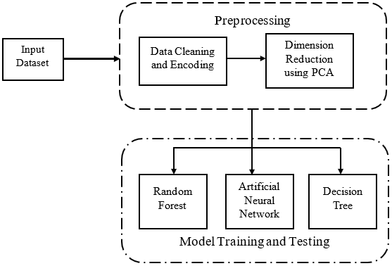
In this study, a comparison of three classification methods for employee performance prediction is presented. An employee dataset obtained from Kaggle was used as the input to the system. Figure 1 depicts the proposed system’s overall structure.
Dataset
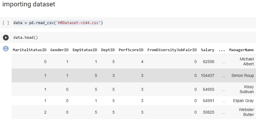
This study uses the Human Resource Dataset obtained from the Kaggle repository. Employee data with a range of attributes make up the dataset. The CSV is based on a fictitious business. Names, dates of birth, marital status, gender, date of hire, department, grounds for termination, active or terminated status, position title, salary rate, manager name, and performance score are all included in the data collection. The dataset contains 36 attributes, each with 311 distinct values and no missing values [16]. The human resource dataset was loaded into Google Collaboratory IDE. Figure 2 shows the loaded dataset comprises 36 attributes with 311 unique values and no missing values. The target value is the performance attribute. This attribute has an employee that fully meets or exceeds the performance and those that do not meet the required performance (noted as PIP - needing Performance Improvement Plan). The view of the table on the paper is limited. The performance column could not be shown in the screenshot captured.
Data Preprocessing
This stage seeks to convert unstructured data into a form that machine learning systems can use. The steps include data cleaning/encoding and Dimension reduction using Principal component analysis (PCA).
Data Cleaning/Encoding
A preliminary analysis of the dataset’s data instances and properties shows that preprocessing is needed since attributes are of different types (binary, numerical and nominal). Since the classification methods will be operating on numeric data, non-numeric data are classified (or transformed) to a numeric value [1], [17].
Principal Component Analysis
Principal component analysis was also applied as a preprocessing step. By condensing a high number of variables into a smaller group that retains the majority of the data from the larger collection, Principal Component Analysis (PCA), a dimensionality reduction approach, decreases the dimensionality of large data sets. The key concept behind PCA is to execute a linear mapping of data from a high-dimensional domain to a lower-dimensional space. The data’s variance is maximized [18]. The algorithm creates a new set of attributes by combining the existing ones.
For formalization purposes, let \(X=x_1, x_2,.., x_n\) be the dataset, in which each \(x_i\) refers to a data instance. An instance \(x_i\) described by \(D\) attributes is defined by the feature vector \(x_{1,1},..,x_{i,D}\). The following are some key points to remember about PCA steps:
Center the data by subtracting the values of each data instance \(x_i\) by the mean \(\mu\) according to \(z_i=x_i - \mu\)
Knowing that \(Z=z_1, z_2,..,z_n\) compute the covariance matrix using \(\sum=Z^TZ\)
Compute the eigenvalues \(\delta_i = \delta_1,..,\delta_D\) and the eigenvectors \(V\) of the covariance matrix using spectral decomposition that is presented \(\sum=VAV^{-1}\), where \(A\) is a diagonal matrix with eigenvalues on the diagonal and zeroes elsewhere, and \(V\) is the matrix of eigenvectors. The eigenvalues on the diagonal of \(A\) correspond to the columns in \(V\) so that the first element of \(A\) is \(\lambda_1\), and the associated eigenvector is the first column of \(V\), and so on.
In order of decreasing difficulty, there is a need to select the eigenvalues and the \(k\) eigenvectors associated with the \(k\) biggest eigenvalues, where \(k\) is the reduced space’s number of dimensions (low-dimensional space). The primary components, which depict a linear transition from the initial attribute space to a new space with uncorrelated attributes, are defined by the eigenvectors. This is expressed by \(PC_1 = c_{1,1}x_1 + c_{1,2}x_2 + .. + c_{1,D}x_D\) in which \(PC_1\) denotes the \(l-th\) principal component (PC), \(x_1, .. , x_D\) are the data attributes and \(c_{1,1}, .. , c_{1,D}\) refer to the coefficients of \(PC_1\). The outputs from PCA, i.e., the eigenvalues, the principal components, and their coefficients are useful for analyzing patterns in data. In many Education Data Mining (EDM) tasks, the identification of the main components affecting students’ performances is essential. As the original representation of the data (original attributes) was transformed into principal components, an analysis of the coefficients of principal components and the amount of explained variance was to obtain implicit knowledge from educational data. Such coefficients express the correlation of each variable to the principal component, and its signal and magnitude are taken into account for interpreting the data patterns [18].
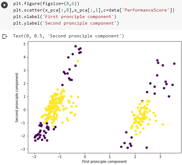
Principal component analysis, a data pre-processing technique, was
used to compress the dataset while retaining relevant information.
Several columns were observed to have no significance to the model, so
it is dropped from the dataset. Some of the columns dropped include
employee_Name, EmpID, Salary,
PositionID, Position, State,
Zip, DOB, Sex,
Date of Hire, Date of Termination. Out of the
36 attributes fed as features into the PCA, 20 attributes retained the
principal components. The dataset’s principal component of the test and
train sets are shown in Figure 3.
Classification Algorithms
The algorithms compared for classification in this study include Decision Trees, Random Forests, and Artificial Neural Networks.
Decision Tree
The decision tree is a supervised Machine Learning technique that is non-parametric. A particular kind of target variable that is widely used in the classification of issues is a decision tree [19], [20]. It can operate in categorical or continuous modes for input and output variables. When using Decision Trees to address the prediction problem, attribute and class labels are represented by the external node and leaf node of the tree, respectively [20]. According to [21], assuming \(S\) is the training sample set and \(|S|\) is the number of samples contained in the training sample test. The sample is separated into \(n\) classes \(|C_1|,|C_2|,..,|C_n|\). The probability of the sample \(S\) being of the class \(C\) is obtained using Equation [1].
\[ p(S_i)=\frac{|C_i|}{|S|}\]
Taking \(A\) as the number of attribute values, this can be given as \(X(A)\) as a set. We mark as \(S_v\) the subset sample with value \(v\). The entropy of the node sample set \(S_v\) classification is given as \(E(S)\) if the branch node is chosen after attribute \(A\) is selected. To get the expected entropy value caused by \(A\). The weighted sum of the entropy of each subset \(S_v\) is calculated. The entropy can thus be given as presented in Equation [2].
\[ Entropy(S,A)=\sum \frac{|S_v|}{|S|}*Entropy(S_v)\]
The information gain value \(Gain(S,A)\) for the original sample set, \(S\) of attribute \(A\) is given in Equation [3].
\[ Gain(S,A)=Entropy(S)-Entropy(S,A)\]
Where \(Gain(S,A)\) is the compression of entropy expected as a result of the attribute selection of \(A\). The more information is provided by the choice of test characteristic \(A\) for classification, the higher the \(Gain(S,A)\).
Random Forest
With a minor tweak to its settings, the widely used machine learning algorithm random forest is said to produce good results [22]–[24]. It is frequently used in classification because of its simplicity. Numerous decision trees are in a random forest with various sample sets at each node [25]. To obtain an accurate result, the final score from each decision tree is averaged [26], [27]. As a result, a random forest is more reliable than a decision tree because it avoids bias and overfitting by randomly placing different trees in the training set [28]. Suppose there is a training set \(X=x_1,..,x_n\) and responses \(Y=y_1,..,y_n\), bagging \(B\) times repeatedly selects a sample at random with the replacement of the training set and fits trees to the sample in [20].
Artificial Neural Network
Many real-world problems require using a neural network for processing, especially when developing a programming algorithm is challenging. The ANN consists of neurons that act as input to the Neural Network (NN), hidden layers, and output layers. Weights are added for the connection of the neurons [29], [30]. The ANN is trained by showing examples and modifying the weight values of the network according to specified learning rules until the ANN output matches the intended result [31]. A popular ANN is the Multilayer Perceptron (MLP) and it is made up of neurons termed perceptron [32]. MLP is mathematically represented in Equation [4] [33]–[35].
\[ y=f \left( \sum_{z=1}^{n} m_z x_z + b \right)s\]
Where \(y\) is the output, \(x_z\) is input vector \(z=1,..,n\), \(f\) is transfer function, \(m_z\) is the weight vector, and \(b\) is bias. The minimized global error \(E\) using the training algorithm is given in Equation [5].
\[ E= \frac{1}{N} \sum_{n=1}^{n} E_n\]
Taking \(N\) as the number of training patterns, \(E_n\) is the error corresponding to the training pattern \(N\). \(E_n\) is represented in Equation [6].
\[ E_n= \frac{1}{2} \sum_{q=1}^{n} (o_g-t_g)\]
Where \(n\) is the total output nodes, \(g\) is the \(g^{th}\) output node, \(o_g\) is the network output at the \(g^{th}\) output node, \(t_g\) is the target output at the \(g^{th}\) output node.
In the MLP classifier, a \(ReLu\) activation function was used. There were 10 hidden layers in the architecture of the classifier and the MLP was trained to pick the information randomly. The maximum number of iterations was kept at 1000.
Performance Metrics
In this study, the classification algorithms were evaluated and compared using the following metrics: accuracy, specificity, sensitivity, precision, F1-Score, and Matthews correlation coefficient. The matrices are obtained using True Positive (TP), True Negative (TN), False Positive (FP), and False Negative (FN). The TP is when the model properly predicts a positive class. The TN) is when the model properly predicts the negative class. The FP is when the model forecasts a positive class wrongly and the FN is when the model forecasts a negative class erroneously.
Accuracy is measured in classification tasks as the proportion of correct predictions made by the model out of all guesses, as presented in Equation [7] [13], [36], [37].
\[ Accuracy= \frac{TP+TN}{TP+FP+FN+TN}\]
The statistic used to assess a model’s capacity to forecast true negatives in each accessible category is called specificity, which is expressed mathematically in Equation [8] [35].
\[ Specificity = \frac{TN}{FP+TN}\]
Recall (also called sensitivity, true positive rate, or TPR) is the ratio of the number of positive instances identified correctly to the number of instances with a positive class. It is obtained using Equation [9] [6], [37], [38].
\[ Recall = \frac{TP}{TP+FN}\]
Precision (given in Equation [10]) is a metric that indicates the percentage of correct predictions made compared to the total number of forecasts made [36].
\[ Precision = \frac{TP}{TP+FP}\]
F1-Score is the balanced average of the recall and precision of the classifier. It is calculated using Equation [11] [18], [39].
\[ F1 = \frac{2TP}{2TP+FP+FN}\]
Results and Discussion
In this section, the output of each major step of the system is examined. The output of the evaluation of the classification algorithms is also stated and compared with each other. A final comparison is made with other similar systems. For each algorithm, we divided the pre-processed dataset into a testing and training set. The dataset is divided into two halves, with 80 percent used for training and 20 percent used for testing. The training dataset is used to determine (or learn) the best variable combinations for building a strong predictive model. The testing dataset is used to evaluate the final model’s fit on the training dataset objectively.
Decision Tree Classifier
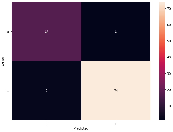
After the data was fed into the Decision Tree classifier, it gave an accuracy of 0.97. The accuracy, precision, specificity, sensitivity, and f1-score of the decision tree after testing are shown in Table 1. Figure 4 shows the confusion matrix.
| Performance Measures (%) | Artificial Neural Network | Random Forest | Decision Tree |
|---|---|---|---|
| Accuracy | 0.9894 | 0.9787 | 0.9681 |
| Precision | 1.0000 | 1.0000 | 0.9867 |
| Specificity | 1.0000 | 1.0000 | 0.9444 |
| Sensitivity | 0.9868 | 0.9737 | 0.9737 |
| F1 Score | 0.9934 | 0.9866 | 0.9801 |
Artificial Neural Network
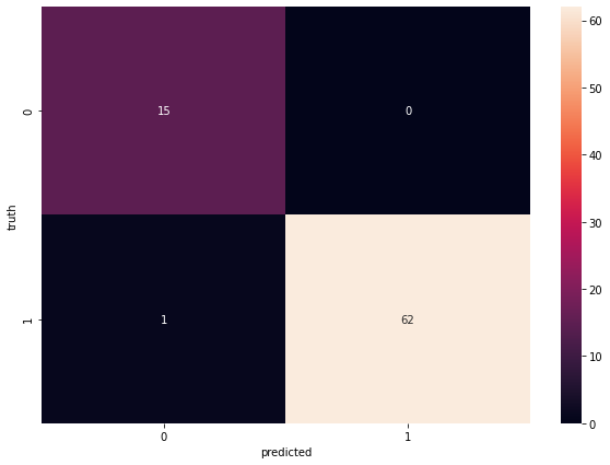
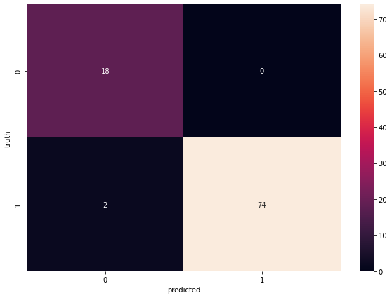
The type of neural network used was the multilayer perceptron. A feedforward artificial neural network called a multilayer perceptron produces a number of outputs from a set of inputs (MLP). The result of the Neural Network showed an accuracy of 0.99. The accuracy, precision, specificity, sensitivity, and f1-score of the decision tree after testing are shown in Table 1. Figure 5 shows the confusion matrix.
Random Forest
When the dataset was fed into the random forest classifier, it had a classification accuracy of 0.97. The confusion matrix of the random forest classifier is shown in Figure 6. The accuracy, precision, specificity, sensitivity, and f1-score of the decision tree after testing are shown in Table 1.
Comparison of Decision Tree and Artificial Neural Network
The ROC Curve shows how well the categorization thresholds performed. The real positive rate is plotted against the false positive rate on the curve. The Receiver Operating Characteristics (ROC) Curve for Neural Network, Decision Tree, and Random Forest is shown in Figure 7.
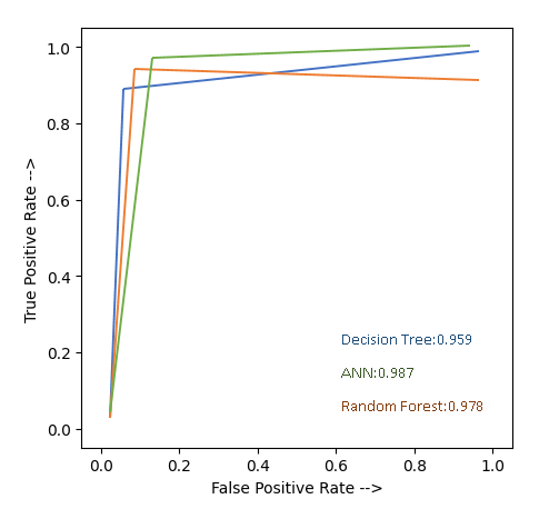
In this study, Table 1 shows the evaluation result and the ANN outperformed others with an accuracy of 98.72%. Also, although DT had better accuracy than RF, the Specificity and Precision of RF were observed to be higher than DT. In fact, in terms of Specificity and Precision, ANN and RF have the same score. This shows that the ability of RF to predict true negatives is the same as that of ANN.
Conclusion and Recommendation
In this study, Data mining techniques were used to construct a classification model for predicting employee performance using a real dataset from the Kaggle Repository. The Decision Tree (DT), Artificial Neural Network, and Random Forest techniques were utilized to create the classification model and select the most relevant parameters that positively affect performance. It was observed after testing that although ANN outperformed RF in terms of performance, they were evenly matched in specificity and precision. This shows that the ability of ANN and RF to accurately predict true negatives is the same. The performance of DT was lower than the other methods. This was expected as RF is a combination of several DTs. However, due to the simplicity of DT, its performance was still impressive. Among the three methods compared, ANN would be recommended for performance prediction of employee performance in organizations with ample resources and in situations where critical decisions would be made on the result. In organizations with medium resources, RF would be recommended for use. In small organizations and in situations where the outcome of the predictions would not be critically used, DT is recommended.
Authors' Information
Jide Kehinde Adeniyi received a B.Sc. degree in Computer Science from Adamawa State University, Nigeria. He holds his M.Tech. in Computer Science from the Federal University of Technology, Nigeria. He obtained his doctoral degree in the Department of Computer Science, University of Ilorin, Nigeria. His interest range various topics in biometrics, computer vision, security, artificial intelligence, and machine learning
Abidemi Emmanuel Adeniyi is currently a lecturer and researcher in the Department of Computer Sciences at Precious Cornerstone University, Nigeria. His area of research interest is information security, the computational complexity of algorithms, the internet of things, and machine learning. He has published quite a number of research articles in reputable journal outlets.
Yetunde Josephine Oguns is currently a Ph.D. student at Ajayi Crowther University, Nigeria. She obtained her Master’s Degree in Computer Science from the University of Ibadan, and her Bachelor of Technology (B.Tech.) in Computer Science from the Federal University of Technology Akure, Nigeria. She also obtained Higher National Diploma and National Diploma in Computer science respectively from Computer Science Department, The Polytechnic Ibadan, Nigeria, where she currently lectures. Her research interest includes Artificial Intelligence, the Internet of Things, Data Science, and Smart Solutions. She is a member of the Computer Professional association of Nigeria (CPN), the Nigeria Computer Society (NCS), the International Association of Engineers (IAENG), and the Organization for Women in Science for the Developing World (OWSD).
Gabriel Olumide Egbedokun is a Ph.D. student in Computer Science at Ajayi Crowther University Nigeria. He obtained M.Sc and B.Sc. in Computer Science from Ajayi Crowther University and the University of Ibadan respectively. His research interests include Data Science, Natural Language Processing, Modeling, and the Internet of Things
Kehinde Douglas Ajagbe is a lecturer in the Department of Computer Science, Kogi State College of Education, Nigeria. He currently serves as the Head of the Department of Computer science and Deputy Director of the College ICT Centre. He earned a Bachelor of Technology Degree (B.Tech.) in computer science from the Federal University of Technology, Nigeria in 2001. In 2013, obtained Postgraduate Diploma in Education (PGDE) from Benue State University Makurdi, Nigeria. He received Masters of Science (M.Sc) degree in Computer Science from the University of Ilorin, Nigeria in 2014. His research interests are in Distributed computing, IoT, and Machine learning. He has many publications in highly rated databases.
Princewill Chima Obuzor is a Ph.D. Candidate in Data Mining at the University of Salford in the Manchester United Kingdom. He obtained a Master’s in Databases and Web Based systems at the University of Salford and a B.Sc. with Distinction at V. Dahl East Ukrainian National University in Luhansk, Ukraine. His research interests are in Machine Learning and Artificial Intelligence, Data Science, Process Mining, and Blockchain Technologies. He is a member of the British computer society (BCS) in the UK.
Sunday Adeola Ajagbe is a Ph.D. candidate in the Computer Engineering Department at the Ladoke Akintola University of Technology (LAUTECH), Nigeria. He obtained M.Sc and B.Sc in Information Technology and Communication Technology respectively at the National Open University of Nigeria (NOUN), and he also has PGD in Electronics and Electrical Engineering at LAUTECH. He has earlier obtained HND and ND in Electrical and Electronics Engineering at The Polytechnic, Ibadan, Ibadan, Nigeria. His specialization includes Artificial Intelligence (AI), Natural language processing (NLP), Information Security, Data Science, the Internet of Things (IoT), Biomedical Engineering, and Smart solutions. He is licensed by The Council Regulating Engineering in Nigeria (COREN) as a professional Electrical Engineer. He is a Member of the International Association of Engineers (IAENG), and the Nigeria Computer Society (NCS). He is a student member of the Institute of Electrical and Electronics Engineers (IEEE). He has published quite a number of research articles in reputable journal outlets such as Springer, ScienceDirect, IEEE, IET Press, and Taylor & Francis press.
Authors' Contributions
Jide Kehinde Adeniyi participated in conceptualization, review, validation, writing of the original draft, and supervision.
Abidemi Emmanuel Adeniyi participated in methodology, software, and coding.
Yetunde Josephine Oguns participated in the literature search and writing of the original draft.
Gabriel Olumide Egbedokun participated in the literature search.
Kehinde Douglas Ajagbe participated in the literature search and writing of the original draft.
Princewill Chima Obuzor participated in the Software, Project administration, and coding.
Sunday Adeola Ajagbe participated in review editing and supervision.
Competing Interests
The authors declare that they have no competing interests.
Funding
No funding was received for this project.