Introduction
According to IEEE Software Engineering Vocabulary [1], Software Engineering (SE) is the application of a systematic, disciplined, quantifiable approach to the development, operation, and maintenance of software; that is, the application of engineering to software. Software is produced through a development process that aims to meet the needs of its users. Such process is one of SE’s main objects of study, for which several process models or lifecycles have been proposed, some of them more linear from the construction point of view, while others are iterative in nature [2]. In the latter, software construction occurs simultaneously with other activities such as design and planning.
Many iterative methodologies, such as Unified Process’, Scrum or Feature Driven Development - FDD, propose to make a prioritization of the requirements. This task aims to achieve an ordering over the requirements according to their priority level. This prioritization helps when choosing what requirements will be implemented in each iteration, and it is useful to make decisions during iteration management.
The criteria taken into consideration in requirement prioritization usually varies between methodologies. For instance, in Scrum the prioritization is realized by the Product Owner by means of Product Backlog ordering [3]. Although no attribute is specified in Scrum Guide, it is expected that the ordering is performed exclusively by value (i.e., the value or importance that the correspondent functionality can bring to the client), since the Product Owner represents the client in the Development Team. In others like the Rational Unified Process (RUP), both technical risk and business value are taken into account [4].
However, in practice, other criteria are taken into consideration when planning an iteration. Besides business value and technical risk, reusability may be of particular interest as it allows effort to be saved for future functionalities. Another criterion usually considered is the requirements’ capacity to be postponed if delays occurs in other tasks (a practice known as slack in Extreme Programming [5]). It seems reasonable then to introduce all attributes that may be relevant to sort the requirements.
Nevertheless, as the number of attributes considered in the process increases, comparisons become not only less significant, but also more difficult to perform. This phenomenon is produced by the curse of dimensionality [6], that is, more attributes introduce the impossibility of a-priori comparing requirements that are non-dominated (without using further preference information).
On the other hand, multiple decision makers are usually involved in the prioritization process. In OpenUP (Open Unified Process), for instance, it is recommended that the whole team participate in the Iteration Planning [7]. Again, in Scrum, Sprint Planning is a ceremony in which the entire team participate and may also invite other people to attend in order to provide advice [3].
Ultimately, the iteration planning is based on the expert judgement of the development team through an unstructured decision process where discussion and consensus among its members are key components. Therefore, such a process has artisanal and heuristic characteristics that are far from the systematic, disciplined and quantifiable approach that defines SE. For all this, it can be concluded that the prioritization process is typically multi-criteria and multi-person [8].
Furthermore, an additional aspect that characterizes the prioritization process is that the valuations assigned to each requirement’s attributes suffer from the cone of uncertainty’s effects [9]. That is, such valuations are only estimates of the real values of the attributes, which will become more certain as time passes. This uncertainty comes from various sources and can take different forms, such as nonspecificity (several alternatives on which it has not yet been decided, for example, scope or design), imprecision (lack of definite or sharp distinctions between categories, for example, when estimating a feature’s complexity as Low or Moderate), strife (conflicting evidence or judgements, for instance, from multiple experts), among others [10]. In this sense, the use of estimates in the form of numbers or classic qualitative ordinal scales constitutes a methodologically questionable approach, since it implicitly assumes that such attributes are known with certainty. Moreover, the use of probability theory can also be questioned, as only can cope with only one dimension of uncertainty (conflict) [11]. Consequently, it is necessary to make use of a framework that takes into consideration the multiple dimensions of uncertainty present in the requirement prioritization process.
Fuzzy Logic [12] offers a theoretical framework that allows to capture the imprecision of expert judgements through the use of linguistic labels, which represent fuzzy sets or numbers. These labels can be ordered by a nonreciprocal fuzzy preference relation [13], where a label \(s_i\) is preferable to another \(s_j\) to a certain degree that varies between 0 (\(s_i\) is not preferable at all to \(s_j\)) and 1 (\(s_i\) is at least as preferable as \(s_j\)), admitting intermediate values. These labels can be used as values of the different attributes of the requirements and obtain orders from them. Fuzzy Logic also offers tools for decision-making in contexts with multiple objectives and multiple decision makers [10], so it is judged as a highly valuable tool in solving problems such as requirement prioritization.
This work extends the proposal made in [14] and [15] and is structured as follows. Section 2 presents the proposed method for approaching the prioritization process. Therein, subsection 2.1 introduces the Fuzzy Linguistic Labels, 2.2 describes the relevant aggregation operators used, and 2.3 specifies the prioritization algorithm that produces the requirements ordering from the imprecise evaluations of multiple experts across multiple dimensions or attributes. Section 3 presents the case of study used to test the approach and an experimental study about the impact of changing the t-norm in the prioritization process. Section 4 contrasts this proposal with related works. Finally, section 5 collects the most relevant conclusions and identifies improvements that will be addressed in future work.
Proposed method
Fuzzy linguistic labels
This article presents a method that uses only ordinal information through a tuple of linguistic labels sorted by their index.
Let \(S\) be a finite and totally ordered set of labels used to indicate preferences with odd cardinality, where \(\forall s_i, s_j \in S, s_i \geq s_j \rightarrow i \geq j\). The semantic of each linguistic term \(s_i\) is given by the ordered structure. For example, \(S^1 =(Low, Middle, High)\).
Among the benefits associated with this ordinal fuzzy linguistic approach, two of them are primal. First, its simplicity, since this technique works directly taking into consideration the order of the labels in \(S\). Secondly, the fact that linguistic assessments are approximations that are handled when it is impossible or unnecessary to obtain more accurate values [16]. Thus, the experts can provide evaluations for each requirement on each dimension of interest using this tool without focusing in selecting a numeric value, resulting in an intuitive and effortless task.
Given \(E\), a set of experts, \(P\), a set of requirements to be prioritized, and \(D\), a set of dimensions or objectives to be evaluated by the experts, the method must be provided with \(|E|\) matrices \(O^{|P|\times |D|}\), where each \(o_{k}(l,m) \in S\) represents the opinion of expert \(e_k \in E\) on how well the requirement \(p_l \in P\) meets the dimension (criterion) \(d_m \in D\).
Additionally, each expert \(e \in E\) can be linked to an importance degree using also the ordinal scale \(S\) so their opinion will be ponderated accordingly. The same can be done with the evaluated dimensions, so each dimension \(d \in D\) weighs differently in the prioritization process.
Aggregation
In order to aggregate the \(|E|\) aforementioned experts’ opinions, an Induced Ordered Weighted Averaging Operators (IOWA) is used to generate a single general matrix with the combined opinions of all the experts. More specifically, in this work we use the majority guided linguistic IOWA (MLIOWA) operator proposed in [16] because it solves common problems related to the semantic of aggregated linguistic values, and it is a majority guided operator, so the weights used in the aggregation process are induced considering the majority of values in the expert importance degree vector, allowing the multiple experts’ evaluations to be aggregated in a single one for each requirement in each dimension. Nonetheless, it is important to note that any other IOWA operator with similar characteristics can be used, for instance, based on another aggregation criterion than that of the majority.
First, let \(Neg\), \(Max\) and \(Min\) be a unary operator and two binary operators respectively, defined on a linguistic set \(S = \{s_1, s_2, \dots, s_{|S|}\}\) as presented in Equations 1 to 3.
\[\label{} Neg(s_i) = s_{ |S| - i + 1 }\]
\[\label{} Max(s_i, s_j) = s_{ max(i,j) }\]
\[\label{} Min(s_i, s_j) = s_{ min(i,j) }\]
The MLIOWA operator is a function \(\varphi^I_Q: (S\times S)^{|E|}\rightarrow S\), defined as follows, where \(I\) is the vector of importance related to the experts, and \(Q\) is a linguistic fuzzy quantifier representing the concept of majority in the aggregation presented in Equation 4.
\[ \varphi^I_Q( (I_1, p_1), \cdots, (I_{|E|}, p_{|E|})) = s_k\]
with \(s_k \in S\) and \(k\) as presented in Equation 5.
\[ k = round(\sum_{i=1}^{|E|} w_i \cdot ind(p_{\sigma(i)}))\]
such as:
\(ind: S\rightarrow \{1,...,|S|\}\) such that \(ind(s_i) = i\)
\(\sigma :\{1,...,|S|\}\rightarrow \{1,...,|S|\}\) is a permutation such that \(u_{\sigma(i+1)} \geq u_{\sigma(i)}, \forall i = 1,...,|E|-1\).
the order inducing values \(u_i\) are calculated using the importance degrees \(I_i\) as shown in Equations 6 and 7.
\[ u_i = \frac{sup_i + ind(I_i)}{2}\]
\[ sup_i= \sum_{j=1}^{|E|} sup_{ij} | sup_{ij} = \begin{cases} 1 & \text{if } | ind(I_i) - ind(I_j)| < \alpha \in \{ 1,...,|S|\}\\ 0 &\text{otherwise} \end{cases}\]
and, lastly, the weighting vector \(\bar{w}\) calculated using the order inducing values as shown in Equation 8.
\[ w_i = \cfrac{ Q\left(\cfrac{u_{\sigma(i)}}{|E|}\right)}{ \sum_{j=1}^{|E|} Q\left(\cfrac{u_{\sigma(j)}}{|E|}\right)}\]
For further information about the MLIOWA operator, see the original publication [16].
Prioritization algorithm
In a previous work, an algorithm for multi-criteria requirement prioritization was presented [14]. In this work, a variation of that work that uses only linguistic labels and includes multiple expert opinion is shown.
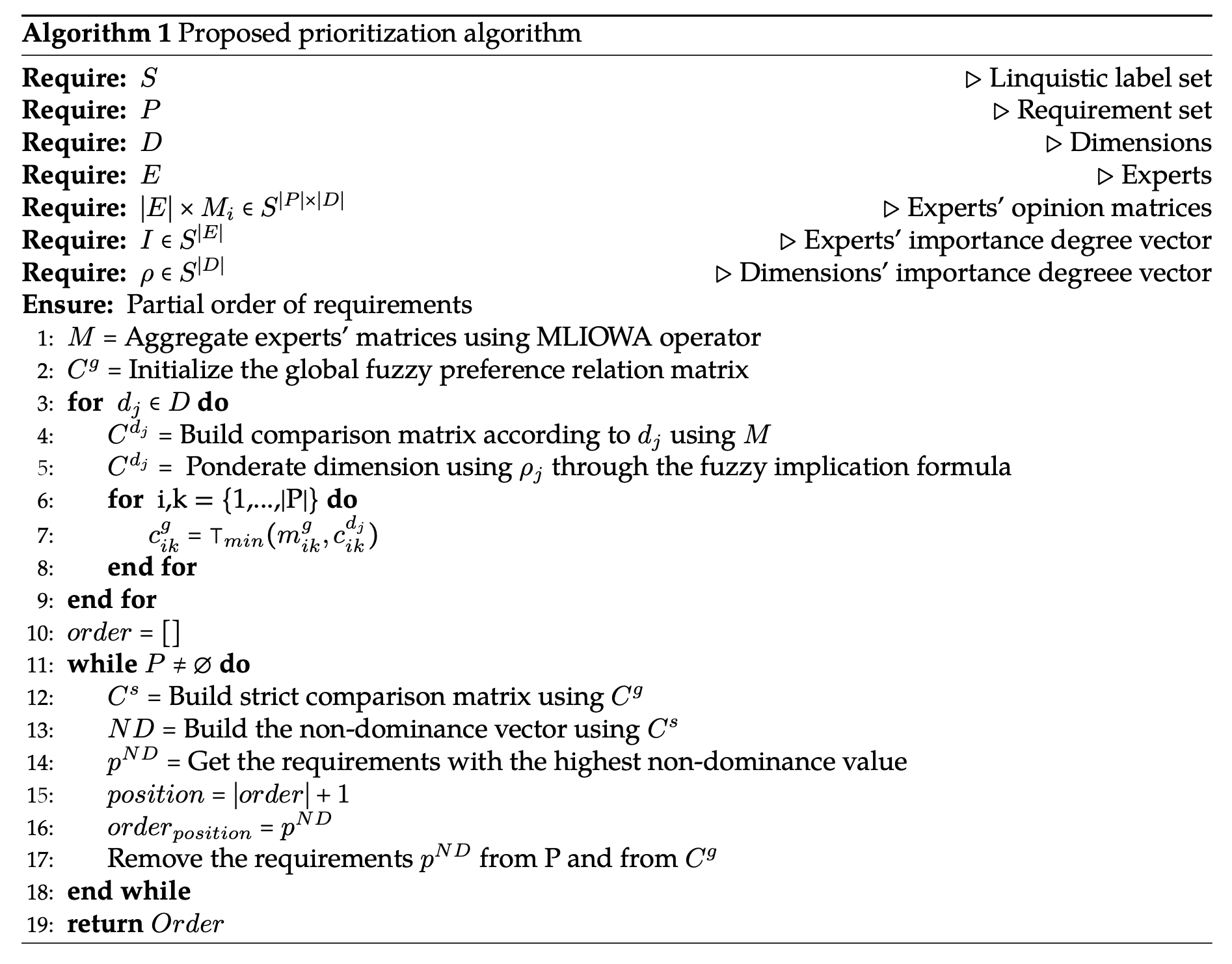
Given a set of linguistic labels \(S\), a set of experts \(E\), a set of requirements to be prioritized \(P\), a set of dimensions or criteria \(D\), \(|E|\) matrices \(O^{|P|\times |D|}\), just as was defined in Section 2.1, and also given an expert importance degree vector \(I \in S^{|E|}\) and a criteria weight vector \(\rho \in S^{|D|}\), the steps of the algorithm are the following:
First, the experts’ opinions must be aggregated using the MLIOWA operator as stated in Section 2.2 using as input the \(|E|\) matrices \(O_i\) and the experts importance degree vector \(I\), producing a matrix \(M^{|P|\times |D|}\) with the aggregated experts’, where each \(m_{ij} \in S\) represents the aggregated opinion of the set of experts about requirement \(p_i \in P\) in relation to the dimension \(d_j \in D\).
The next step is to build a comparison matrix for each dimension using as input the matrix \(M\). For a specific dimension \(d_j \in D\), the comparison matrix \(C^{d_j}\) represents the fuzzy preference relation \(R_{d_j} \subseteq P \times P\), where \(\mu_{R_{d_j}}\), defined as shown in Equation 9, is the degree to which the requirement \(p_i \in P\) is at least as good as \(p_k \in P\) according to the criterion \(d_j\).
\[\small c^{d_j}_{ik} = \mu_{R_{d_j}} (p_i, p_k) = \begin{cases} 1 & \text{if } ind(m_{ij}) \geq ind(m_{kj}) \\ 0 & \text{if } ind(m_{ij}) < ind(m_{kj}) - \beta \\ 1 - \cfrac{|ind(m_{ij}) - ind(m_{kj})|}{\beta + 1} & \text{otherwise} \\ \end{cases}\] \(\text{with }\beta \in \mathbb{N}, 0 < \beta < |S|\). Given a dimension \(j\), when \(ind(m_{ij}) \ge ind(m_{kj})\), i.e., when \(p_i\)’s label is at a position greater or equal to the position of \(p_k\)’s label, then \(p_i\) is at least as preferable to \(p_k\) in maximum degree regarding dimension \(j\) (e.g., at \(S^1\), Middle is at least as good as Low at grade 1). Further, when \(ind(m_{ij}) < ind(m_{kj}) - \beta\), i.e., when the label of \(p_i\) is at more than \(\beta\) positions of \(p_k\), then \(p_i\) is not at all preferable to \(p_k\) (e.g., at \(S^1\), with \(\beta = 1\), Low is at least as preferable as High at grade 0). Lastly, when the position of \(p_i\)’s label is at \(\beta\) or fewer positions than the position of \(p_k\)’s label, then it is still possible that \(p_i\) is preferable to \(p_k\), but in a lesser degree, proportional to the distance between positions (e.g., at \(S^1\), with \(\beta = 1\), Low is as preferable as Middle at grade 0.5). Such possibility exists due to the imprecision in the experts’ evaluations. Hence, \(\beta\) is a parameter that reflects the overlapping between the fuzzy linguistic labels and depends on the characteristics of the addressed problem.
Then, these preference relations represented by each comparison matrix need to be weighted considering the criteria weight vector to obtain the pondered preference relations. To do this, an implication approach similar to the one presented by [17] can be used according to Equation 10, where \(\rightsquigarrow\) is the fuzzy implication symbol and \(\bot\) is the fuzzy T-conorm used to define it. This would be the fuzzy version of the logical equivalence \(p \rightarrow q \equiv \lnot p \lor q\)
\[\label{} \mu^{\rho_j}_{R_{d_j}} (p_i, p_k) = \rho_j \rightsquigarrow \mu_{R_{d_j}} (p_i, p_k) = \bot (1-\cfrac{ind(\rho_j)}{|S|}, \mu_{R_{d_j}} (p_i, p_k))\]
Then, the global fuzzy preference relation \(R_g\) is the intersection
\[R_g = \bigcap\limits_{j=1}^{|D|} R^{\rho_j}_{d_j}\] using the classic T-norm Min as shown in Equation 11.
\[\label{} \mu_{R_g}(p_i, p_k) = \displaystyle \top \min \limits_{d_j \in D}^{} \{\mu^{\rho_j}_{R_{d_j}}(p_i, p_k)\}\]
The global fuzzy preference relation is used then to build a new relation: the strict global fuzzy preference relation \(R_{s}\). The complement of \(\mu_{R_{s}}(p_i, p_k)\) (equation 12) represents the degree to which \(p_i\) does not dominate \(p_k\), and can be used to calculate the degree to which an alternative \(p_k\) is not strictly dominated by any other alternative. This last fuzzy set is called fuzzy non-dominance set and is calculated as shown in Equation 13 [13].
\[\label{} \mu_{R_{s}}(p_i, p_k) = \max\{\mu_{R_g} (p_i, p_k) - \mu_{R_g} (p_k, p_i), 0\}\]
\[\label{} \mu_{R_{ND}}(p_k) = \displaystyle \min\limits_{p_i} \{1-\mu_{R_{s}}(p_i, p_k)\} = 1- \displaystyle \max\limits_{p_i} \{\mu_{R_{s}}(p_i, p_k)\}\]
The best alternative \(p^{ND} \in A\) is the requirement with the highest membership degree to the fuzzy non-dominance set \(R_{ND}\). Also, when this value is equal to 1, the decision is said to be non-dominated and non-fuzzy.
Borzęcka [18] proposes using the non-dominance fuzzy set to make the prioritization, but this may not be appropriate if there are alternatives that are not strictly dominated by others. For example, if there are 3 alternatives a, b and c, such that a dominates b, b dominates c and, transitively, a dominates c, b and c would have their membership degree equal to 0 making them equally preferable according to [18], which is not true.
In order to solve this problem, the most preferable solutions \(p^{ND}\) can be removed from the set, then the membership function of the remaining alternatives to the strict global fuzzy preference relation can be calculated again and finally their non-dominance degree. This procedure is repeated until there is no alternative left to be prioritized.
This method fits problems with either small or large numbers of requirements because it is possible to compose a single global fuzzy relation from an arbitrary number of dimensions. For this, fuzzy preference relations are used to evaluate multiple criteria with different degrees of importance in order to classify the alternatives considering the stakeholders’ opinions, weighted by their relevance. Then, a decreasing order of the solutions is obtained taking into consideration all the aforementioned aspects.
The structure of the algorithm is described in Algorithm 1.
Case study
In order to illustrate how the proposed method works, a proof of concept using a generated dataset is shown below as a weak form of validation [19]. The dataset consists of five experts’ opinions about 10 requirements related to a Content Management System (CMS) (see Table 1) evaluated on 3 different dimensions: Complexity degree of implementing the requirement, Degree of Reusability of the implementation and Importance to Costumer. This set of dimensions gives better results in the requirement prioritization process according to [20].
| ID | Requirement description |
|---|---|
| 1 | Customize the User Interface. |
| 2 | Add Content Editor and content approver role. |
| 3 | Provide a portal to the Content provider with options. |
| 4 | Email notifications to be sent to content provider. |
| 5 | Conversion of the content to Digital format. |
| 6 | Quality check of the content. |
| 7 | Check Content format. |
| 8 | Apply security over the content. |
| 9 | Create package. |
| 10 | Create poster for advertisements. |
The requirement set, the dimensions and the first expert evaluations were obtained from [14], [20] (see Table 2). The rest of the opinions were generated arbitrarily. An implementation of this method and the data used for this experiment are publicly available, and the link to the repository can be found in the Availability of Data and Material section of this article.
Firstly, in all the cases the fuzzy linguistic label set that was used is S, described below. In this case, the label “VL” means Very Low, “L” means Low, “M” means Medium, “H” stands for High and lastly “VH” stands for Very High. However, it is important to note that the semantic of each label is given by its position in the tuple, as was mentioned in Section 2.1.
\[S = (s_1: \text{``VL''}, s_2: \text{``L''},s_3: \text{``M''},s_4: \text{``H''},s_5: \text{``VH''})\]
| Requirement | Complexity | Reusability | Importance |
|---|---|---|---|
| 1 | M | L | H |
| 2 | M | VH | VH |
| 3 | VH | M | H |
| 4 | VL | VL | VL |
| 5 | M | H | H |
| 6 | VH | VH | H |
| 7 | L | L | L |
| 8 | VL | M | VL |
| 9 | VL | L | L |
| 10 | L | VL | VH |
Additionally, the expert importance degree vector \(I\) and the criteria weight vector \(\rho\) used were the ones described below:
\[\begin{aligned} I = & (i_1: \text{``M''}, i_2: \text{``VH''}, i_3:\text{``M''}, i_4:\text{``M''}, i_5:\text{``M''}) \\ \rho = & (\text{Complexity}: \text{``VH''}, \text{Reusability}: \text{``M''}, \text{Importance}: \text{``M''})\end{aligned}\]
Using the aforementioned input, the first step of the algorithm aims to aggregate the experts’ opinions into a single general matrix. To do this, the MLIOWA operator is used. Hereunder, the calculations for the element \(m_{11}\) are presented as an example, corresponding to the requirement 1 and the criterion “Complexity,” being the experts’ opinions for this pair the following:
\[(e_1: \text{``M''}, e_2: \text{``M''}, e_3: \text{``L''}, e_4: \text{``H''}, e_5: \text{``M''})\]
The support \(sup_i\) for each expert importance degree was calculated according to equation 7, considering \(\alpha = 1\), getting the vector \(sup = (4, 1, 4, 4, 4)\) as result. The first element of the vector was calculated with Equation 14, and the rest of the elements were calculated equally.
\[\label{} sup_1 = \sum\limits_{j=1}^{5} sup_{1j} = 1+0+1+1+1 = 4\]
The next step aims to get the order inducing value vector \(u\), calculated with Equation 15 according to Equation 6.
\[ u = \left (\cfrac{4+3}{2}, \cfrac{1+5}{2}, \cfrac{4+3}{2}, \cfrac{4+3}{2}, \cfrac{4+3}{2} \right) = (3.5, 3, 3.5, 3.5, 3.5)\]
The vector \(u\) induces the order shown in Table 3 and allows to get the weights to weigh the experts’ opinions using Equation 8. In this case, the fuzzy quantifier “most of,” Q, was defined by the parameters (0.3, 0.8). These weights can be seen in the same table mentioned above.
| \(\sigma\) | Expert | u | \(\, \, \mu_Q \, \, \,\) | \(w_i\) |
|---|---|---|---|---|
| 1 | \(e_1\) | 3.5 | 0.8 | 0.21 |
| 2 | \(e_3\) | 3.5 | 0.8 | 0.21 |
| 3 | \(e_4\) | 3.5 | 0.8 | 0.21 |
| 4 | \(e_5\) | 3.5 | 0.8 | 0.21 |
| 5 | \(e_2\) | 3 | 0.6 | 0.15 |
Lastly, the experts’ were aggregated according to the induced order using the weights calculated before, using Equation 16.
\[\label{} k = round(\sum\limits_{i=1}^{5} w_i \cdot ind(p_{\sigma_i}) )\]
\[\begin{aligned} k & = round( 0.21 \cdot ind(\text{H}) + 0.21 \cdot ind(\text{M}) + 0.21 \cdot ind(\text{M}) + 0.21 \cdot ind(\text{L}) + 0.15 \cdot ind(\text{M}) ) = \\ & = round( 0.21 \cdot (4 + 3 + 3 + 2) + 0.15 \cdot 3) = round(2.97) = 3 \end{aligned}\]
Then, the aggregated value for the requirement 1 evaluated on the criterion “Complexity” is \(s_3: \text{``M''}\). The whole aggregated matrix is shown in Table 4.
| Requirement | Complexity | Reusability | Importance |
|---|---|---|---|
| 1 | M | L | H |
| 2 | M | VH | VH |
| 3 | H | M | H |
| 4 | VL | VL | VL |
| 5 | M | H | H |
| 6 | VH | VH | H |
| 7 | L | L | L |
| 8 | VL | M | VL |
| 9 | VL | L | L |
| 10 | L | VL | VH |
After aggregating the experts’ opinions, the comparison matrices for each dimension were calculated using Equation 9 (with \(\beta = 1\))and then weighed using the Equation 10 with the vector \(\rho\). Then, the global fuzzy preference relation was determined as the intersection of the three aforementioned comparison matrices. The result of this process can be seen as follows.
\[\small C^g = C^{\text{Complexity}} \cap C^{\text{Reusability}} \cap C^{\text{Importance}} = \left( \begin{array}{cccccccccc} 1&.4&.5&1&.4&0&1&.5&1&.5\\ 1&1&.5&1&1&0&1&1&1&1\\ 1&.4&1&1&.5&.4&1&1&1&.5\\ 0&0&0&1&0&0&.5&.4&.5&.4\\ 1&.5&.5&1&1&0&1&1&1&.5\\ 1&.5&1&1&1&1&1&1&1&.5\\ .4&.4&0&1&.4&0&1&.5&1&.4\\ 0&0&0&1&0&0&.5&1&.5&.4\\ 0&0&0&1&0&0&.5&.5&1&.4\\ .5&.4&0&1&.4&0&.5&.4&.5&1 \end{array} \right)\]
Lastly, the strict comparison matrix was computed, and then the partial order was generated by iteratively calculating the non-dominance vector and selecting those requirements with the biggest non-dominance membership value. The non-dominance vector calculated in each iteration as well as the non-dominated requirements are shown in Table 5. The resulting order, then, is the one shown in the "Selected" column, being the ones in the first row more preferable than the one in the second row and so on. If there are two or more requirements in a row, that means those requirements are equally preferable.
| Requirements | ||||||||||||
| i | Order | 1 | 2 | 3 | 4 | 5 | 6 | 7 | 8 | 9 | 10 | Selected |
| 1 | 1 | 0.0 | 0.5 | 0.4 | 0.0 | 0.0 | 1.0 | 0.0 | 0.0 | 0.0 | 0.4 | 6 |
| 2 | 2 | 0.4 | 1.0 | 0.9 | 0.0 | 0.5 | - | 0.0 | 0.0 | 0.0 | 0.4 | 2 |
| 3 | 3 | 0.4 | - | 1.0 | 0.0 | 1.0 | - | 0.0 | 0.0 | 0.0 | 0.5 | 3, 5 |
| 4 | 5 | 1.0 | - | - | 0.0 | - | - | 0.4 | 0.5 | 0.0 | 1.0 | 1, 10 |
| 5 | 7 | - | - | - | 0.4 | - | - | 1.0 | 1.0 | 0.5 | - | 7, 8 |
| 6 | 9 | - | - | - | 0.5 | - | - | - | - | 1.0 | - | 9 |
| 7 | 10 | - | - | - | 1.0 | - | - | - | - | - | - | 4 |
The results are consistent with the results obtained in [14]: when a single expert is provided, the two methods are equivalent.
\[\small C^s = \left( \begin{array}{cccccccccc} 0 &0&0&1&0&0&.6&.5&1&.0\\ .6&0&.1&1&.5&0&.6&1&1&.6\\ .5&0&0&1&0&0&1&1&1&.5\\ 0&0&0&0&0&0&0&0&0&0\\ .6&0&0&1&0&0&.6&1&1&.1\\ 1&.5&.6&1&1&0&1&1&1&.5\\ 0&0&0&.5&0&0&0&0&.5&0\\ 0&0&0&.6&0&0&0&0&0&0\\ 0&0&0&.5&0&0&0&0&0&0\\ 0&0&0&.6&0&0&.1&0&.1&0 \end{array} \right)\]
T-norm comparison
As mentioned in [15], the prioritization method proposed in this work uses the T-norm min to intersect the comparison matrices calculated for each evaluated dimension (Algorithm 1, step 7). Nonetheless, any other T-norm can be used.
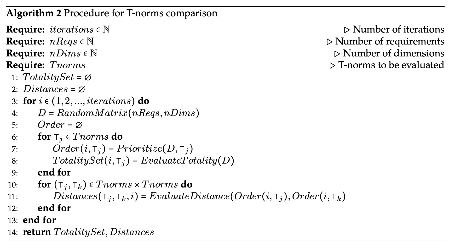
In order to understand if the selection of the t-norm used in this step produces a relevant impact in the result of the prioritization process, three different t-norms were compared by using random data matrices following the procedure specified in Algorithm 2.
This procedure uses input matrices generated randomly by taking values from the aforementioned vector \(S\) of linguistic labels. The number of requirements was constant and equal to 100 and the number of dimensions varied from 3 to 9, in order to understand whether the behavior associated with each T-norm depends on this parameter. With each configuration 500 comparisons were performed.
It is also important to note that this randomly generated matrices simulate an aggregated matrix or the input matrix provided by just one expert, due to the lack of impact of this parameter in the objective of study. For the same reason, the dimensions were considered to have the same importance degree, so the weighting process was not performed.
On the other hand, the t-norms considered in this work were the t-norm Min (\(\top_{Min}\)), also called the Gödel t-norm, for being the de-facto standard in the literature, the t-norm Product (\(\top_{Prod}\)) for allowing the variables to interact with each other, and the Łukasiewicz T-norm (\(\top_{Luk}\)), for differ in the way the variables interact by using a summative formula. These t-norms are calculated respectively as shown in Equations 17, 18 and 19.
\[\label{} \top_{Min}(a,b) = \min(a,b)\]
\[\label{} \top_{Prod}(a,b) = a \cdot b\]
\[\label{} \top_{Luk}(a,b) = \max(0, a+b-1)\]
The procedure begins by generating in each iteration a random matrix of expert’s opinions using the parameters mentioned before. Then, for each t-norm the prioritization process was carried on as specified in the previous sections. Then, the totality degree of each generated order was calculated. This metric aims to get the degree to which an order is closer to be total as the ratio between the length of the longest chain (totally ordered set) that is subset of the evaluated order, and the length of its lineal extension, which is the same as the number of requirements.
Then, for each pair of t-norms, a distance was calculated between the orders generated by each one of them for a specific input matrix. This metric aims to find the average difference between the position of the requirements in both orders through the function shown in Equation 20, where \(R\) is the set of requirements, and \(Pos(x, O)\) is a function that returns the position of the requirement \(x\) in the order \(O\).
\[\label{} Distance(O_{\top_j}, O_{\top_k}) = \cfrac{\sum\limits_{x \in R} | Pos(x, O_{\top_j}) - Pos(x, O_{\top_k}) | }{|R|}\]
As a result of the whole procedure, a set of totality values for each t-norm and a set of distance values between each pair of t-norms paired by input matrix was obtained. The distribution of these values can be seen in Figure 1.


Using the Wilcoxon signed-rank test [21], the non-parametric version of the paired t-test, it was tested if there are significative differences between the distribution of the totality variable for each considered t-norm. The results can be seen in Table 6.
| Hypothesis | Wilcoxon Statistic | P-value | RBC | CLES |
|---|---|---|---|---|
| \(H_0: Totality(Prod) \leq Totality(Min)\) | 2871928.0 | 0.0 | 0.999992 | 0.883074 |
| \(H_A:Totality(Prod) > Totality(Min)\) | ||||
| \(H_0: Totality(Prod) \leq Totality(Luk)\) | 2881200.0 | 0.0 | 1.0 | 0.970211 |
| \(H_A: Totality(Prod) > Totality(Luk)\) | ||||
| \(H_0: Totality(Min) \leq Totality(Luk)\) | 2875044.0 | 0.0 | 0.997276 | 0.877522 |
| \(H_A: Totality(Min) > Totality(Luk)\) |
According to the results, there is \(88.30\%\) of probability for the totality variable to be higher if the Product t-norm is used instead of the Min t-norm, \(97.02\%\) of probability to be higher if the Product t-norm is used instead of the Łukasiewicz t-norm, and a \(87.75\%\) to be higher if the Min t-norm is used instead of the Łukasiewicz t-norm, according to the common language effect size measure (CLES) [22] and the Rank-biserial correlation measure [23], as can be seen in the aforementioned table.
On the other hand, as can be seen in Figure 1, the totality degree decreases with the number of dimensions, specially using the min and the Łukasiewicz t-norm. With the product t-norm, the totality value increases with low dimensionality but decreases after 5 dimensions. This behavior could be produced due to the curse of dimensionality. If the number of dimensions is low, the extra dimensions could help the method to break ties, but if more dimensions are considered, the method could have problems in the comparison process. This hypothesis will be tested in future works.
Furthermore, the distance between paired solutions consistently increases for the pairs Łukasiewicz and min, and Łukasiewicz and product. Thus, we could expect solutions to be different if Łukasiewicz t-norm is used instead of any of the others. For the pair product t-norm and min t-norm, the solutions are more similar for higher dimensionality, having small totality degree. This also can be seen in Figure 2, which shows how the probability of the totality value for the product t-norm to be higher than the value for the min t-norm decreases with the number of dimensions, so the orders tends to be more similar to each other, which also can be seen in the Figure 1. Additionally, the dispersion of the distance variable for this pair also increases, which does not occur for the other two pairs.

In consequence, we can expect the orders obtained using the product t-norm to be more total than the ones obtained with the min and the Łukasiewicz t-norms. In addition, the higher the dimensionality, the more partial these orders are. Also, by using the Łukasiewicz t-norm we cannot ensure results similar to the ones obtained using the min or the product t-norm, but these last two t-norms tends to produce more similar results instead.
| Position | |||||||||||
| T-norm | 1 | 2 | 3 | 4 | 5 | 6 | 7 | 8 | 9 | 10 | Totality |
| Min | 6 | 2 | 3, 5 | - | 1, 10 | - | 7, 8 | - | 9 | 4 | 0.7 |
| Product | 6 | 2 | 3, 5 | - | 1 | 10 | 7 | 8,9 | - | 4 | 0.8 |
| Łukasiewicz | 6 | 2 | 3, 5 | - | 1 | 10 | 7 | 8,9 | - | 4 | 0.8 |
These results can be used to choose the more appropriate T-norm according to both the characteristics of the problem and the characteristics of the decision-maker. More total orders, obtained using the product t-norm, may be preferred to the partial ones, for example, when trade-offs between objectives are allowed, while the opposite may be preferable when the decision-maker wants to break the ties according to their personal experience, specially when the number of criteria is low. This can be achieved, for example, by using the min t-norm.
Table 7, for example, shows different orders for the requirements used in the case study presented in Section 3, each of which was obtained using a different T-norm and considering all the evaluated dimensions of equal importance degree. It can be noted that the T-norm min produced an order that is more partial than the one obtained using the product t-norm, being both orders consistent with each other.
Differences arise in pairs of requirements \(p_1\) and \(p_{10}\), and \(p_7\) and \(p_8\). In the last case, using the min t-norm, \(p_7\) and \(p_8\) are equally preferable (i.e., neither dominates the other), whereas with product and Łukasiewicz t-norms, \(p_7\) has priority over \(p_8\). This is because product and Łukasiewicz t-norms allow some interactivity between the criteria. Particularly in this case, \(p_7\) is slightly superior to \(p_8\) in Complexity (\(c^{Complexity}(p_7, p_8) = 1\), \(c^{Complexity}(p_8, p_7) = 0.5\)) and Importance (\(c^{Importance}(p_7 , p_8) = 1\), \(c^{Importance}(p_8, p_7) = 0.5\)), while \(p_8\) is slightly superior in Reusability (\(c^{Reusability}(p_7, p_8) = 0.5\), \(c^{Reusability}(p_8, p_7) = 1\)). Aggregating the criteria using the min t-norm, \(c^g(p_7, p_8) = min(1, 0.5, 1) = 0.5\) and \(c^g(p_8, p_7) = min(0.5, 1, 0.5) = 0.5\), thus the strict relation values are \(c^S(p_7, p_8) = c^S(p_8, p_7) = 0\), i.e., \(p_7\) and \(p_8\) do not dominate each other. However, it could be considered that, since \(p_7\) is slightly superior to \(p_8\) in two of the three criteria, the former should have priority over the latter. This type of compensation can be taken into account if, for instance, the product t-norm is used. In such a case, aggregating the criteria yields \(c^g(p_7, p_8) = 1 \cdot 0.5 \cdot 1 = 0.5\) and \(c^g(p_8, p_7) = 0.5 \cdot 1 \cdot 0.5 = 0.25\), and thus \(c^S(p_7, p_8) = 0.25\) and \(c^S(p_8, p_7) = 0\), i.e. \(p_7\) is preferable to \(p_8\). Similar results can be achieved with Łukasiewicz’s t-norm. A similar analysis can be done for requirements \(p_1\) and \(p_{10}\) (\(p_1\) is slightly superior in Complexity and Reusability, while \(p_{10}\) is slightly superior in Importance).
Lastly, all the tests performed in these evaluations are available in the Availability of Data and Material section.
Related work
According to Bukhsh et al [24], only a few articles uses fuzzy logic for requirement prioritization in software engineering. These studies differ from our proposal as describe hereunder.
Lima et al [25] suggested a framework that uses fuzzy linguistic terms parameterized using fuzzy numbers. In contrast, our methods do not need to use fuzzy numbers due to the fact that the semantics of each label is associated to its order in the fuzzy linguistic label set. Additionally, our method allows integrating multiples decision makers or experts, which is not considered in the previously mentioned proposal. This also occurs in [26]. The authors designed a method for requirement prioritization easy to use and implement but do not consider multiple experts’.
On the other hand, Achimugu et al [27] considers the opinion of multiple stakeholders parameterized with triangular fuzzy numbers as in [25] but do not consider multiple objectives or criteria as our method does.
Then, Franceschini et al [28] proposes a method for fusing multiples orders of priority, given by multiple experts with different degrees of importance. This method allows the stakeholders not to include into their order all the requirements, which is a tremendous advantage if the experts do not have the same degree of expertise on the different evaluated criteria. However, this method uses as input an order of requirements per expert, which is not the case of our algorithm that uses the experts’ opinions about the requirements instead.
Moreover, search-based approaches, like presented by Tonella et al [29], propose to perform a prioritization incorporating order constraints, for instance, of technical precedence or business priority nature. However, the resolution method, based on an interactive genetic algorithm, does not help in the initial definition of such constraints, and our method could be used to that effect. Furthermore, the proposal of [29] is based in the interaction with a single decision maker, while our method allows incorporating the opinion of multiple decision makers or experts.
Finally, the problem of grouping requirements and assigning them to software iterations or releases can be viewed as a prioritization. This problem has been formulated as an optimization problem and is known as the Next Release Problem (NRP) or Release Planning (RP). There are many variants, both mono [30] and multi-objective [31]. However, as in the approach mentioned in the previous paragraph, information about the priority or value of requirements is often used as a measure of merit or quality to guide the search. Similarly, the results of our approach can be used as parameters for the NRP and RP problems.
To sum up, the algorithm proposed in this article allows the user to generate a partial order of a set of requirement based on multiple experts’ opinions with different importance degrees on multiple criteria, that also are weighed. Moreover, the proposed method takes as input fuzzy evaluations using fuzzy linguistic labels, which allows the experts to provide their opinions in a more familiar way. The semantics of the linguistic labels is given by their position in the ordered fuzzy linguistic label set, so they do not depend on the definition of fuzzy numbers.
The method is easy to implement and use. This can be seen in the implementation annexed to this article, making it highly applicable in the industry, which is a common limitation remarked in [24].
Conclusion
This work presents a method for requirement prioritization that uses the opinions of many experts on many decision criteria, expressed using fuzzy linguistic labels. The opinions are aggregated using a majority guided linguistic IOWA considering weights for each expert, and then, the requirements are compared based on the aggregated experts’ opinions on the evaluated dimensions, which are also weighed by their importance. Moreover, the weights linked to the criteria and to the experts are expressed using also fuzzy linguistic labels.
The proposed method was demonstrated using a case of study that works as a initial form of validation. The algorithm was implemented in such a way that the user only has to provide the opinions and basic configurations to use it. This is a very desirable property. In future works, an empirical study has to be performed to complement the one presented in these pages, in order to understand how the proposal works in a real context with real users.
In contrast to previous works, this article also presents an initial comparison of the different T-norms that can be used in the process, particularly in the intersection of each evaluated dimension. This study shows significant differences in the degree to which an order is more linear depending on the t-norm that was used to obtain it. Nonetheless, the study was performed without considering different importance degree for each dimension. Because of the use of a t-conorm in the weighting process that usually is associated with a t-norm, the results may vary if this extra factor is considered. This consideration remains for future works, as well as using different metrics to evaluate the obtained orders.
Finally, other improvements to be made in the future includes allowing the experts not to give an opinion for all the evaluated dimensions, considering consensus metrics in the prioritization process, using and comparing other IOWA operators, and using a different linguistic label set for each dimension.
Acknowledgments
The authors want to thank Tomás Casanova and Kevin-Mark Bozell Poudereux for proofreading the translation, and to the anonymous reviewers for their valuable comments and suggestions.
Authors' Information
Giovanni Daián Rottoli is Information Systems Engineer and Ph.D. candidate in Computer Sciences. He is professor and researcher in the Computational Intelligence and Software Engineering research group from the Universidad Tecnológica Nacional, Facultad Regional Concepción del Uruguay (Argentina).
Carlos Casanova is Ph.D. in Engineering and Information Systems Engineer. He is professor and main researcher in the Computational Intelligence and Software Engineering research group from the Universidad Tecnológica Nacional, Facultad Regional Concepción del Uruguay (Argentina).
Authors' Contributions
Giovanni Daián Rottoli made the experiment design and execution and participated in the results analysis as well as writing the manuscript.
Carlos Casanova made the algorithm design and participated in the results analysis as well as writing the manuscript.
Competing Interests
The authors declare that they have no competing interests.
Funding
National Technological University Project SIUTICU0005297TC: “Preference-based Multi-objective Optimization Approaches applied to Software Engineering.” Argentina.
Availability of Data and Material
GdRottoli/RequirementPrioritization: RP v1.1.0. 2021. DOI: https://doi.org/10.5281/zenodo.5327643
GdRottoli/RequirementPrioritizationExperiments_TnormsComparison: Min-Prod-Luka Comparison (V1.0). DOI: https://doi.org/10.5281/zenodo.5771120