Introduction
Nowadays, the Graph Neural Networks (GNNs) proposed in 2009 [1] has been widely used for processing the data in the non-Euclidean space, especially the graph data. Because of the powerful processing capabilities for the unstructured data, GNNs are widely used in many areas such as social networks [2], [3], drug discovery [4], and recommendation [5], [6]. The existing GNN models can be roughly classified into four categories, one of which is Convolutional Graph Neural Networks (ConvGNNs) [7]. ConvGNNs can be further classified into two categories, spectral-based ConvGNNs and spatial-based ConvGNNs. Graph Convolution Network (GCN) is a typical spectral-based ConvGNN model [8], [9].
To efficiently train GCN and improve the generalization ability of GCN for new nodes, the Graph SAmpling based INductive learning meThod (GraphSAINT) [10] is proposed. GraphSAINT uses a sampling method called the subgraph sampling method to generate a serial of subgraphs from the whole graph and then build a GCN on the subgraph. This subgraph sampling method alleviates the problem of the neighbor explosion so that the number of neighboring nodes no longer increases exponentially with the number of layers in GraphSAINT. Moreover, GraphSAINT has a stronger processing capability for large graphs by sampling multiple subgraphs from the original dataset to construct minibatch for training compared with the Graph SAmple and aggreGatE (GraphSAGE) algorithm [11]. In general, nodes with a broader influence on each other can be selected to form a subgraph with a higher probability. However, the subgraph sampling method applied in GraphSAINT leads to a different node sampling probability and introduces bias into the mini-batch estimator, which makes the training more difficult. To deal with this problem, the normalization techniques are proposed and applied in [10] to make sure that the feature learning will not give priority to the more frequently sampled nodes. Therefore, GraphSAINT can achieve a better accuracy score on the classification task.
However, experiments show that the stability problem appears during training when GraphSAINT is applied to deal with the link prediction task [12], [13] on the citation dataset of the standard Open Graph Benchmark (OGB) [14]. Unlike the node classification task, the main task of link prediction is to predict whether there is a link between two nodes in a network. This stability problem during training means that the normalization techniques in [10] are insufficient to guarantee the training quality for link prediction. So the training loss may fall into non-convergence, which indicates that the value of the training loss will suddenly rise and remain unchanged. Training stability is important to the development of GNNs.
We can get some inspiration in training stability from the CNN training methods. Stochastic gradient descent and its variants such as momentum [15] and Adagrad [16] have been widely used to train the neural networks. As the number of neural network layers gradually increases, changes to the neural network parameters will amplify [17]. When constantly adapting to the new distribution, the distributions of layers’ inputs present a problem called covariate shift [18], which is bad for neural network convergence. Ioffe and Szegedy presented the Batch Normalization (BN) to reduce the internal covariate shift and accelerate the convergency of the deep neural nets [17]. This technique makes use of the mean and variance to normalize the data values over each mini-batch, which brings a higher learning rate and drops the Dropout [19]. Besides BN, Layer Normalization (LN) is also widely used among normalization techniques [20], but it uses a different normalization method from BN. However, the effective normalization techniques have drawn little attention in GNNs due to the fewer network layers [7]. As the graph becomes larger and larger, the GNN models are more complicated, which leads to the stability problem during training. Thus, the application of the normalization techniques is of great significance to the robustness in training on large graphs. Besides, the tricks of GNNs have drawn more attention in recent years. The presence of the tricks helps improve the accuracy of the GNN algorithms significantly on the OGB datasets [21], [22]. However, the role of GNN tricks on model stability needs to be further verified.
Therefore, to solve the stability problem in the training process of the traditional GraphSAINT for the link prediction task, we propose the improved GraphSAINTs by adjusting two normalization techniques, that is BN and LN, and one GNN trick to the training and inference process of the traditional GraphSAINT based on the citation dataset of OGB in this paper. By applying the three techniques to the model, we eliminate the instability of the traditional GraphSAINT during training successfully. Moreover, we also realize a reduction in the training time and improve the accuracy under the premise of maintaining the original link prediction accuracy with the help of the improved GraphSAINTs. We validate the effectiveness of our methods by the citation dataset of OGB.
Inspired by [23], the paper organizes as follows: Firstly, section 2 is the related work about the traditional GraphSAINT, especially its sampling strategy. Besides, we briefly present two normalization techniques, which is BN and LN, and a GNN trick; Next, section 3 describes our improved GraphSAINTs and the processes of training; Then, section 4 shows the related experiment results based on the citation dataset of OGB; At last, conclusions are given in Section 5.
Related work
The Sampling Strategy of the traditional GraphSAINT
Since GCN aggregates one-hop neighbors’ information via the adjacent matrix [8], [9], it has a low generalization ability as mentioned in section 1, that is, GCN can not deal with the problem of adding a new node to a graph. If we want to obtain the node representation of the new node, we need to update the adjacent matrix and re-train the GCN model to update the model parameters. Therefore, GraphSAGE is proposed to improve the generalization ability of GCN [11]. GraphSAGE makes use of the neighbor sampling strategy and defines a new learnable aggregation function to aggregate neighbor nodes’ information. The process of generating a target node embedding avoids using the adjacent matrix and the time of retraining the model.
Instead of the neighbor sampling strategy, GraphSAINT achieves the sampling of large images by proposing a sampler called SAMPLE [10]. This sampling method is called the subgraph sampling method, which can help GraphSAINT deal with the neighbor explosion problem. Besides, similar to GraphSAGE, GraphSAINT also has the generalization ability for new nodes.
The sampler can preserve the connectivity characteristic of the graph. Therefore, bias in the mini-batch estimation will be almost inevitably introduced by the sampler. Therefore, the determination of sampling probability is the critical step to realizing the subgraph sampling method. In [10], the sampling probabilities of each node, edge, and subgraph are all well-estimated by deriving the corresponding formulas. Furthermore, the subgraphs obtained by sampling will be used for the GraphSAINT training.
The typical normalization techniques
Due to the change of the distributions during training, the internal covariate shift appears in a deep network. So the normalization techniques are used to eliminate this shift and achieve a faster training time [24], [25]. In the following, we mainly introduce two normalization techniques, which is BN and LN.
BN presented in [17] is a typical normalization technique for mini-batch. BN follows the mathematical statistics: Firstly, the mean is calculated over a mini-batch; Next, the variance is calculated by the mean; Then, each data over a mini-batch can be normalized by subtracting the mean and then divided by the variance; Finally, the scale and shift parameters are learned for each data point over a mini-batch. In BN, the mean and the variance are calculated for different neuron unit inputs, and the inputs in the same batch have the same mean and variance. Therefore, BN is sensitive to the size of the batch size. Since the mean and the variance are calculated on one batch, if the batch size is too small, the calculated mean and variance are not enough to represent the entire data distribution.
Different from BN, LN calculates the mean and variance of the input of all neuron units in a specific layer of the deep network to perform the normalization operation and does not depend on the batch size. Therefore, the input of the neuron units in the same layer in LN has the same mean and variance, and different input samples have unequal means and variances.
Free Large-scale Adversarial Augmentation on Graphs (FLAG)
As a GNN trick, FLAG is a free large-scale adversarial augmentation on graphs to alleviate overfitting. Different from the existing literature of data augmentation by changing the graph structures, FLAG is conducted in the input node feature space. Standard adversarial training aims to deal with an optimization problem [26]. This kind of optimization problem can be reliably solved by making use of both Stochastic Gradient Descent (SGD) and Projected Gradient Descent (PGD), which may cause the high computational cost and the loss of the model accuracy [27].
FLAG is an adversarial data augmentation on graphs. It can improve the model accuracy and effectively enhance the generalization performance of the model. FLAG mainly achieves data augmentation by adding the small gradient-based adversarial perturbations to the input node features and preserving the graph structures. FLAG is a valuable exploration of the power of adversarial data augmentation on graphs. The general algorithm flow of FLAG is as follows:
Assume that each epoch contains M steps. In each epoch, we first define a perturbation matrix named Pert. Pert that has a gradient is the same shape as the input X and obeys a uniform distribution. Then Pert as perturbations and X are both sent to the model for training. The training has a total of M steps. We manually update Pert according to the gradient of Pert and then clear the gradient of Pert in each step. Finally, after finishing the M steps, we accumulate the M gradient values, and then the model parameters are all updated by the backpropagation.
Methodology
As mentioned in section 1, the original normalization techniques of the traditional GraphSAINT, which are valid for the node classification task, are insufficient to improve the training quality for the link prediction task on OGB. The traditional GraphSAINT needs to be improved to obtain more stable training results. Therefore, we proposed three strategies, including BN, LN, and FLAG, to improve the traditional GraphSAINT and achieve more stable training results. According to the basic principle, the three strategies can be divided into two types: one is the normalization techniques including BN and LN, the other is the GNN trick named FLAG.
Based on the connectivity rules of the nodes, the sampled subgraphs in GraphSAINT can get the edge sampling probability with the minimum variance. In contrast, for node selection, the sampled subgraphs use the random node sampler. So the node feature data of each sampled subgraph do not obey the standard normal distribution. Therefore, the normalization techniques BN and LN are used to normalize the mean and variance of the input data from different perspectives. Besides, as a data augmentation method, the GNN trick named FLAG can enhance the model’s anti-interference ability against the input data by introducing small gradient-based adversarial perturbations into the input node feature data. In the following, we will introduce the two types of improved GraphSAINTs in detail.
The improved GraphSAINTs with the normalization techniques
In this section, we will firstly introduce the first improved GraphSAINT with BN. This improved GraphSAINT is firstly introduced in [28]. Here, we have made some necessary supplementary explanations based on the original version. The improved GraphSAINT with BN realizes that the inputs in the same batch have the same mean and variance. Assume the graph dataset to be processed is a whole graph \(\zeta=(V, \xi)\) with N nodes \(v \in V\), edges \(\left(v_{i}, v_{j}\right) \in \xi\), For the node \(v_{i}\) in a sampled subgraph \(\zeta_{s}\) of \(\zeta\) according to SAMPLE, its feature \(h_{i, s}\) has \(d\) elements. To normalize the input data distribution, the input node feature vector can be normalized by \[\hat{h}_{i, s}=\frac{h_{i, s}-\mu_{s}^{b}}{\sqrt{\left(\sigma_{s}^{b}\right)^{2}}}\] \[\mu_{s}^{b}=\frac{1}{d} \sum_{i=1}^{d} h_{i, s} \quad \sigma_{s}^{b}=\sqrt{\frac{1}{d} \sum_{i=1}^{d}\left(h_{i, s}-\mu_{s}^{b}\right)^{2}}\] where \(\mu_{s}^{b}\) and \(\sigma_{s}^{b}\) are the mean and the variance for the node \(v_{i}\) in the node feature dimension and computed over the training data set. Therefore, after BN, the inputs in the same batch have the same mean and variance.
However, the improved GraphSAINT with LN does not perform the same normalized operation in a batch different from the improved GraphSAINT with BN. This improved method with LN fixes the mean and the variance of the summed inputs in a specific layer of the deep network to reduce the covariate shift. Thus, the LN can be calculated as follows: \[\hat{h}_{i, s}=\frac{h_{i, s}-\mu_{s}^{l}}{\sqrt{\left(\sigma_{s}^{l}\right)^{2}}}\] \[\mu_{s}^{l}=\frac{1}{H} \sum_{i=1}^{H} h_{i, s} \quad \sigma_{s}^{l}=\sqrt{\frac{1}{H} \sum_{i=1}^{H}\left(h_{i, s}-\mu_{s}^{l}\right)^{2}}\] where \(\mu_{s}^{l}\) and \(\sigma_{s}^{l}\) are the mean and the variance over all the hidden units in the same layer, \(H\) is the number of hidden units in a layer. Therefore, the input of neuron units in the same layer in LN has the same mean and variance. Because the different inputs have different means and variances, the input data in the same batch have unequal means and variances.
The whole training process of the improved GraphSAINT with one of the two normalization techniques (BN or LN) is illustrated in Algorithm 1. We can see that when using the two normalization techniques to improve GraphSAINT, a basic flow of the algorithm is roughly the same, and the only thing you need to do is to choose one of the two normalization techniques where the normalization technique is applied. The specific process of Algorithm 1 is as follows:
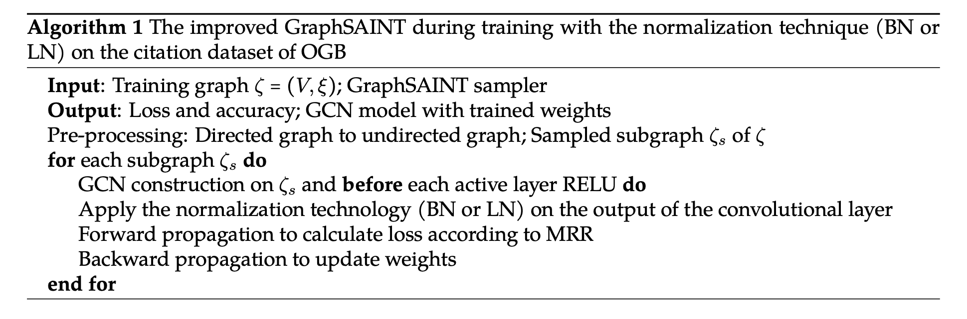
At the beginning of the training, a directed graph is converted to an undirected graph in the stage of the pre-processing on \(\zeta\). And SAMPLE is conducted to obtain the sampled subgraph \(\zeta_{s}\) [10]. Next, an iterative training process is performed via SGD to obtain the updated weights. For each iteration, we use an independent subgraph \(\zeta_{s}\). In the iterative loop, the normalization technique (BN or LN) is applied on the output of the convolutional layer of GCN, which is also the input of the RELU layer. Then the modified GCN on \(\zeta_{s}\) is conducted to rank the missing references and Mean Reciprocal Rank (MRR) is used to calculate the loss in the process of the forward propagation. In MRR, the score of the n\(t h\) matched result is 1/n and the final score is the sum of all scores. Finally, the backward propagation is carried out to update weights.
Besides, although the subgraphs are used for training as mentioned in Section 2.1, the whole graph data are used to obtain the reference result. Therefore, during inference, the normalization operations should be conducted independently.
The improved GraphSAINT with a GNN trick
As mentioned in Section 2.3, the GNN trick named FLAG is a graph data augmentation method that helps relieve overfitting in the training process of a GNN model. FLAG enhances the model robustness by introducing small gradient-based adversarial perturbations into the input node features. The improved GraphSAINT with the GNN trick named FLAG can solve the stability problem in the training process. Besides, it also can improve the accuracy of the traditional GraphSAINT.
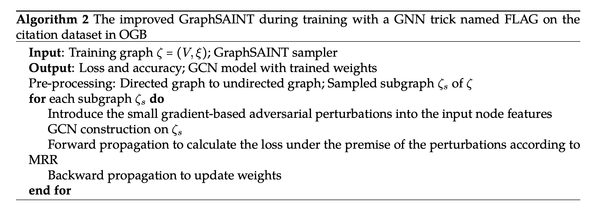
The whole training process of the improved GraphSAINT with a GNN trick named FLAG is illustrated in algorithm 2. We can see that algorithm 2 has the same pre-processing as algorithm 1. Then an iterative training process is also conducted via SGD to update model weights, and each iteration uses an independent subgraph \(\zeta_{s}\). Next, in contrast, algorithm 2 introduces small gradient-based adversarial perturbations into the input node features. Then the input node features with perturbations are fed into the GCN model as input, and GCN construction is performed. Finally, under the premise of the perturbations, the loss can also be calculated according to MRR.
Experiments
In this section, to verify the effectiveness of the improved GraphSAINTs, we choose the link prediction task based on the citation dataset of OGB (ogbl-citation). Before the emergence of OGB, the main characteristic of the existing graph datasets is small. The small graph datasets are far from the web-scale graphs in the real world, which is harmful to the data-driven model research and practical problem solving, and the model trained with such a small dataset is also called a toy model. Such toy models may have similar statistical results on these small datasets, which makes the models hard to distinguish. Besides, such toy models are also hard to extend to large graphs.
There is no doubt that OGB makes toy models a thing of the past. Besides, OGB also gives a unified experimental standard, including the data set division method and the evaluation and verification standard. The datasets contained in OGB can be divided into three groups. Each group corresponds to a specific graph machine learning task. There are three different tasks, which are node classification, link prediction, and graph classification. Because the citation dataset that we choose is used for the link prediction task, citation can also be expanded as ogbl-citation by adding a prefix. The ogbl-citation dataset is a directed graph that represents the citation network between subsets of papers extracted from Microsoft Academic Graph (MAG) [29]. Each node is a paper with 128-dimensional word2vec features that summarize its title and abstract. Each directed edge indicates that one paper cites another paper. All nodes are also accompanied by meta-information indicating the year of publication of the corresponding paper.
The purpose of the link prediction task is to use the currently acquired network data (including structural information and attribute information) to predict which new connections will appear in the network. For the ogbl-citation dataset, the link prediction task is to predict the missing citations that are randomly dropped based on the existing edges. So the model is required to rank the missing references higher than the other existing references. According to this, we choose MRR as the evaluation metric [14]. Besides, the validation set and testing set consist of randomly dropped edges. Naturally, the training set consists of all the rest of the edges.
| GraphSAINT | Training | Validation | Test |
|---|---|---|---|
| official | 0.8626±0.0046 | 0.7933±0.0046 | 0.7943±0.0043 |
| convergence | 0.8690 | 0.8031 | 0.8048 |
| non-convergence | 0.0010 | 0.0010 | 0.0010 |
The results of the traditional GraphSAINT on the citation dataset of OGB are given in Table 1. The official result of GraphSAINT is convergent: the MRR value of the training set is 0.8626 ±0.0046, the MRR value of the validation set is 0.7933 ±0.0046, and the MRR value of the test set is 0.7943 ±0.0043. The official MRR results are the statistical result of 10 RUNs. Therefore, for the convenience of comparison, the hyperparameter named RUN will also be set to 10 in the following experiments.
The bottom two rows in Table 1 are the results of our recurrence experiment of the traditional GraphSAINT. We found that the traditional GraphSAINT will not converge in training with a probability range from 0.1 to 0.4 in the training process. For a RUN where the loss converges, the MRR results are consistent with the official results as shown in Table 1, i.e., the training result can reach about 0.8690, the validation result can reach about 0.8031, and the test result can also reach about 0.8048. The loss curve for a RUN where the loss converges is shown in Figure 1(a). We can see that one RUN contains 200 epochs. Besides, in Figure 1(a), as the epoch increases, the values of the loss gradually decrease overall, although the values of the loss fluctuate slightly in the process of the decline.
The MRR results for a RUN where the loss does not converge are shown in the last row of Table 1, i.e., the training result, the validation result, and the test result are all approximately equal to 0, which means that the MRR results of the run where the loss does not converge are invalid. And the loss curve for a RUN where the loss does not converge is shown in Figure 1(b). We can see that after the 78th epoch, the loss is suddenly and sharply increased to 34.5388 and remains unchanged, which indicates that the loss can not converge afterward. Therefore, some measures need to be taken to help the loss converge and obtain the valid MRR results for the link prediction task.


To deal with the problem of the non-convergence in the training process, three different strategies, which are LN, BN, and FLAG, are applied to improve the traditional GraphSAINT. The results for the improved GraphSAINTs on the citation dataset of OGB are given in Table 2. In particular, we can see that there are four different improved GraphSAINTs. In addition to the three strategies mentioned above, the results of a new combination strategy named BN+FLAG are also shown in the last row of Table 2. As mentioned in section 3, both LN and BN belong to the normalization techniques, while FLAG belongs to the GNN tricks. And we are curious if there are better results for the improved GraphSAINTs after applying the combination of the two types of strategies, that is BN and FLAG. Therefore, the related experiments are added to verify our conjecture. In the following, the results of the four improved GraphSAINTs as shown in Table 2 will be explained in turn. Besides, for each subfigure in Figure 2, a blue dotted line, which is also the loss curve during training of the traditional GraphSAINT with convergence as shown in Figure 1(a), is added. This blue dotted line is used to compare with the loss curve during training of the four improved GraphSAINTs.
| GraphSAINT | Training | Validation | Test |
|---|---|---|---|
| LN | 0.8526±0.0151 | 0.7790±0.0113 | 0.7791±0.0114 |
| BN | 0.9001±0.0014 | 0.8335±0.0020 | 0.8344±0.0023 |
| FLAG | 0.8880±0.0019 | 0.8165±0.0022 | 0.8175±0.0022 |
| BN+FLAG | 0.8997±0.0013 | 0.8349±0.0010 | 0.8364±0.0012 |


At first, LN is listed in Table 2 as an improved strategy for the traditional GraphSAINT, and the three MRR values are shown afterward: the training result can reach 0.8526±0.0151, the validation result can reach 0.7790±0.0113, and the test result can also reach 0.7791±0.0114. After applying the improved GraphSAINT with LN, the loss curve during training is shown by the solid red line in Figure 2(a), where the loss curve is convergent. Moreover, compared with the blue dotted line in Figure 2(a), the solid red line fluctuates more sharply in the first 20 rounds at the beginning of training, but it will be more stable in the later period. In conclusion, we can see that although the improved GraphSAINT with LN has a loss of around 0.015 loss in accuracy compared with the official results of the traditional GraphSAINT, it solves the instability problem in the process of training.
Then, another normalization technique named BN is listed next to LN in Table 2. Compared with the official results for the traditional GraphSAINT, all the three MRR values have an improvement as shown in Table 2: the training result can reach 0.9001±0.0014, the validation result can reach 0.8335±0.0020, and the test result can also reach 0.8344±0.0023. Besides, the loss curve of the improved GraphSAINT with BN during training is shown by the solid red line in Figure 2(b). We can see that the solid loss curve is convergent. Besides, compared with the blue dotted line in Figure 2(b), the improved GraphSAINT with BN has a stable convergence during training and a faster convergence rate. Moreover, because the training time of the improved one with BN is shorter than that of the traditional GraphSAINT, the epoch is 150, as can be seen from the solid red line in Figure 2(b), which is less than 200. Here, it is also clear that the improved GraphSAINT with BN has a better test accuracy than the improved GraphSAINT with LN.
The next row of Table 2 is the experimental results of the improved GraphSAINT with FLAG. Although the improvement is less than the improved GraphSAINT with BN, all the three MRR values still have an improvement compared with the official results for the traditional GraphSAINT as shown in Table 2: the training result can reach 0.8880±0.0019, the validation result can reach 0.8165±0.0022, and the test result can also reach 0.8175±0.0022. Besides, the loss curve of the improved GraphSAINT with FLAG during training is shown by the solid red line in Figure 2(c). Compared with the blue dotted line in Figure 2(c), the improved GraphSAINT with FLAG also has a stable convergence in the training process, whose convergence rate is slightly slower than the improved one with BN. However, since the application of FLAG in the traditional GraphSAINT makes the training time longer, the epoch is 250, as can be seen from the solid red line in Figure 2(c).
The last row of Table 2 is the results of the improved GraphSAINT with a new combination strategy named BN+FLAG. Considering that both BN and FLAG bring an increase in the test accuracy to the traditional GraphSAINT, we conduct such an experiment by using the BN+FLAG combination strategy, and we can see that the training result can reach 0.8997±0.0013, the validation result can reach 0.8349±0.0010, and the test result can also reach 0.8364±0.0012. It’s a pity that the improved GraphSAINT with the BN+FLAG combination strategy has almost the same result of the test accuracy as the improved GraphSAINT with BN, which means that the FLAG strategy hardly improves the test accuracy of the results obtained by the improved GraphSAINT with BN. Besides, the loss curve of the improved GraphSAINT with the BN+FLAG combination strategy during training is shown by the solid red line in Figure 2(d). Although the application of FLAG does not improve the test accuracy of the results, when compared with the blue dotted line in Figure 2(d), we also find that the improved GraphSAINT with the combination strategy achieves a faster convergence rate than the other three improved GraphSAINTs.
Thus, the effectiveness of our improved GraphSAINTs with the three strategies, that is LN, BN, and FLAG, are all verified.
Conclusions
The stability problem in the training process of GNN is crucial. In this paper, we focus on this stability problem and propose the improved GraphSAINTs by applying the two normalization techniques, that is BN and LN, and a GNN trick named FLAG. Experiments show that all the proposed algorithms improve the robustness of the training process of the traditional GraphSAINT and solve the problem of instability during training. Besides, the improved algorithms with BN and FLAG can obtain a better test accuracy. Moreover, the improved algorithms that apply BN also accelerate the convergence of the models. In the future, more attention will be paid to the stability of the GNN models in the process of distributed training for large graph datasets.
Acknowledgments
This research was funded by the Fifth Innovative Project of State Key Laboratory of Computer Architecture (ICT, CAS) under Grant No. CARCH 5403.
Authors’ Information
Yuying Wang received her Ph.D. from the Chinese Academy of Sciences. She is a postdoc at the Institute of Computing Technology, Chinese Academy of Sciences, Beijing.
Huixuan Chi received his Bachelor’s degree from North China Electric Power University. He is studying for a master’s degree at the Institute of Computing Technology, Chinese Academy of Sciences, Beijing.
Qinfen Hao received his Ph.D. from the Chinese Academy of Sciences. He is a professor at the Institute of Computing Technology, Chinese Academy of Sciences, Beijing.
Authors’ Contributions
Yuying Wang participated in planning the manuscript outline, conducting the experiments, and preparing the manuscript.
Huixuan Chi participated in the results analysis and the manuscript preparation.
Qinfen Hao participated in the manuscript preparation.
Competing Interests
The authors declare that they have no competing interests.
Funding
No funding was received for this project.