Introduction
Heart rate variability (HRV) reflects cardiac modulation by sympathetic and vagal components of the autonomic nervous system (ANS) that produces beat-to-beat changes. These changes are analyzed by recording the electrocardiogram (ECG) in whose tracing R waves are identified. The time distance between two consecutive R waves allows obtaining a series of time intervals called cardiotachogram [1] (see Figure 1).

HRV is used as an indicator parameter of the level of cardiovascular health, since it is possible to study the changes in the sympathetic-vagal balance of the cardiac response, resulting in a very useful tool in the study and analysis of the evaluation of individuals who perform sports activities [2], [3].
HRV is a non-invasive method that is used as an indicator of cardiovascular health. In studies of diseases such as diabetes and analysis of cardiovascular and cerebrovascular events, in hypertensive patients, detection of drowsiness, in sleep deprived subjects [4], stressful situations and recently in stress during sports training and in subsequent physiological recovery [5].
HRV studies are classified into long-term studies, with 24-hour records [6] and short-term studies, with 5-minute records [1], [7]–[9].
The increase in the use of mobiles devices allowed the appearance of applications for the analysis of the health status of people, which perform measurements of heart rate, blood sugar, body mass, etc. in short times. Due to this, HRV measurement times should be less than 5 minutes [10] to increase its use as a diagnostic tool in the medical clinic and and also achieve almost real-time measurements [11].
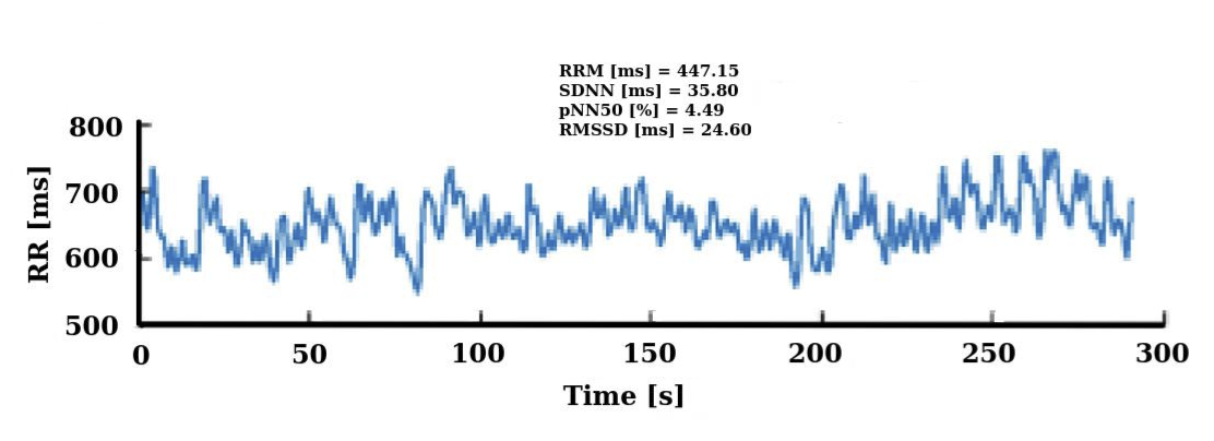
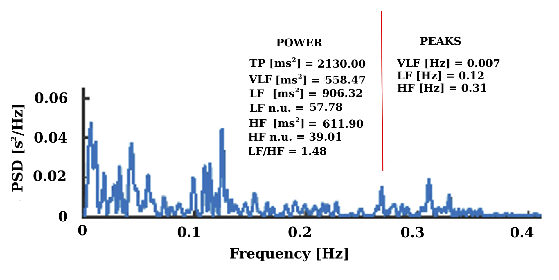
The methods currently used in short-term HRV are geometric and nonlinear analysis [1], and to a greater extent, the time domain analysis using a statistical approach, by means mean of RR intervals (RRM), standard deviation of RR intervals (SDNN), root mean square of the differences between consecutive RR intervals (RMSSD) and percentage value of frequency of successive differences of RR intervals that spanned more than 50 ms (pNN50) (see Figure 2). The frequency domain analysis by power spectral density (PSD) using Lomb periodogram (LP) or Fast Fourier Transform (FFT) for non-equispaced RR series, LP does not require re-sampling of the series, unlike FFT method [12], [13] (see Figure 3). Frequency domain indexes can use the following frequency bands: low frequency (LF) (0.04-0.15 Hz), high frequency (HF) (0.15-0.4 Hz), normalized parameters (LFn.u.), (HFn.u.) and LF / HF ratio [14] (see Figure 3).
The Poincaré domain geometric indexes describe the correlation between consecutive RR intervals [15]. Cross axis, the (SD1) index reflects the short-term variability of heartbeats, related to parasympathetic activity. The (SD2) index reflects the long-term variability, and the (SD2/SD1) ratio is a measure of the relation between the long-and short-term variability similar to the LF/HF ratio by its analogy and properties [4].
From the Poincaré domain, for the assessment of autonomic balance in soccer players [16] proposed two new indexes, of short HRV, a direct index for the evaluation of sympathetic activity SS (stress score) and S/PS (SPS) (sympathetic-parasympathetic ratio) as an indicator of autonomous balance.
The reduction of the recording times of the SS and SPS indicators can increase the use of HRV and particularly its application in the evaluation of sports performance in athletes and also improve the knowledge of the physiological meaning of HRV. Even though, studies suggest minimum lengths of the RR series depending on the index to be calculated [10].
Therefore, this study set out on the one hand, to analyze the behavior of SS and SPS with respect to other time and frequency domain indexes, and on the other hand, to find the minimum recording times for ultra-short HRV required so that the indexes SS and SPS are equivalent to those obtained using short HRV.
Material and Methods
Subjects and design
Overall, twenty-three subjects with a mean age of 23 years voluntarily participated in this study. The subjects were healthy, nonsmokers and had no known cardiovascular diseases and free from any medication. Every subject provided written informed consents for participation in this study before starting it. This study went through ethics approval from the Research Committee at National University of Quilmes, Buenos Aires, Argentina (04/07/2016/No. 3).
HRV analysis
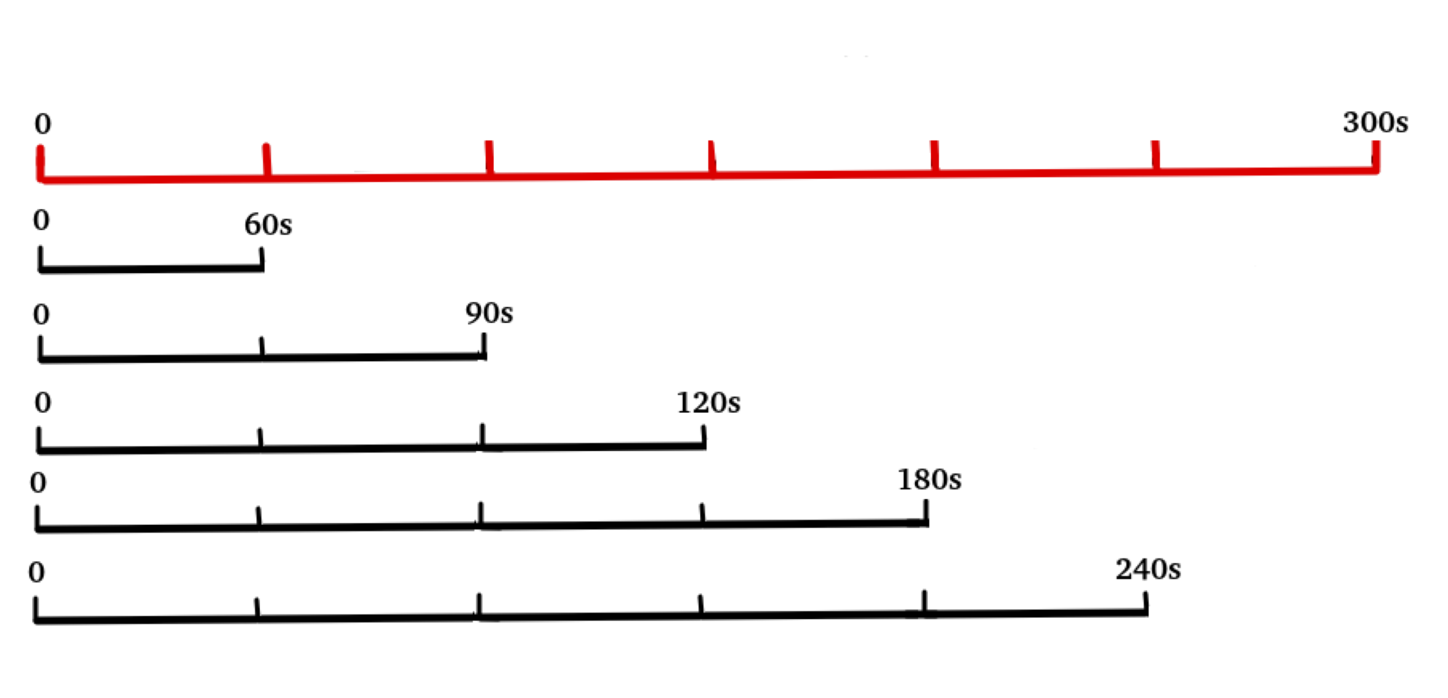
The ECG signal of each subject was obtained in resting position, for 5 min (300 s) and 2 min of stabilization time, with a Holter, by means of the DI lead (DI lead, is formed by placing electrodes between the right arm and the left arm), with a sampling frequency of 225 Hz. ECG signal was processed, using a notch filter was applied to remove interference from the power supply network (50 or 60 Hz), the trends were eliminated by polynomials of order 6 previously adjusted to the signal and then oversampled at 1 KHz, to increase the reliability of measures of the R wave. The modified Pan-Tompkins algorithm was used [17] to detect R peaks, in the QRS complex of the ECG, then the RR time interval series was calculated. In this series, the linear trend and the zero-frequency component were eliminated. To detect atypical beats such as the non-sinus, ectopics, false signal distortions, muscles movement, electromagnetic interference, etc. [1] an impulse rejection filter was used [18], [19]. These atypical beats were replaced by interpolation by another interval whose value was the average of the six RR intervals neighboring the one considered artifact. [20], [21]. For the purposes of the ultra-short HRV analysis, to each 300 s series (the "Gold Standard" (GS) series) time windows of 60, 90, 120, 180 and 240 seconds were extracted (see Figure 4). The HRV analysis was performed in the time domain and the LP was used for the PSD in the frequency domain.
Poincaré Plot
The Poincaré graph presented in Figure 5 is a geometric method where by plotting the RRn interval versus the next RRn+1 interval and adjusting the graph to an ellipse allows us to calculate the HRV indexes [22]. The Poincaré plot method allows to obtain the standard deviation of the instantaneous variability of RR interval, minor axis of the ellipse SD1 (parasympathetic activity) and the standard deviation of the continuous variability of the long-term RR interval, major axis of the ellipse SD2 (sympathetic activity) and the ratio \(SD2 / SD1\) a measure of the relation between the long-term and short-term variability (\(SD21\)) [23]. Equation 1, Equation 2:
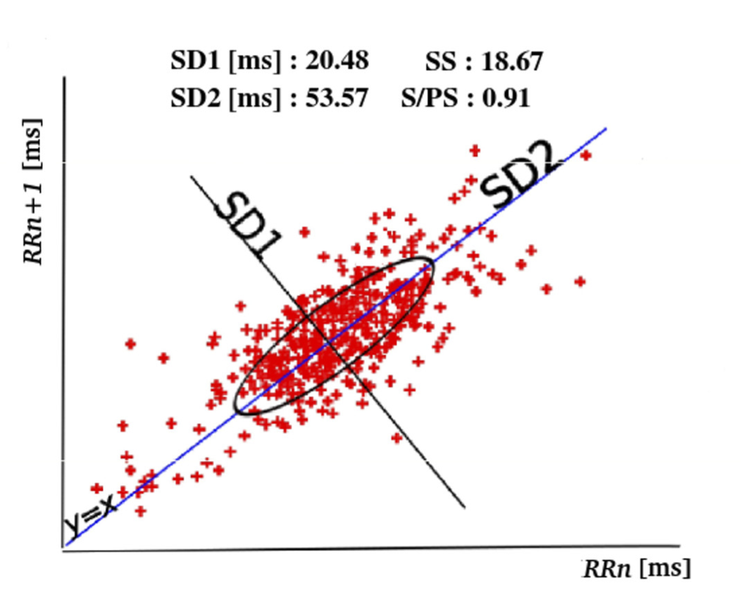
\[ SD1=\sqrt{Var(\frac{RR_n-RR_{n+1}}{\sqrt{2}})}\]
\[ SD2=\sqrt{Var(\frac{RR_n+RR_{n+1}}{\sqrt{2}})}\]
where RRn is a certain interval, RRn+1 is the next interval and Var represents the variance.
The parameters \(SS\) and \(SPS\) were calculated from the Poincaré diagram using the equations proposed by [16], Equation 3 and Equation 4 .
\[ SS = \frac{1000}{SD2}\]
\[ SPS = \frac{SS}{SD1}\]
Signal processing and HRV calculations were developed in GNU Octave.
Statistical analysis
The algorithm proposed by [24], for the situation of lack of normality of some of the series and the concurrent validity criterion applied by [10] were used for the equivalence analysis between the GS series and each of the ultra-short series belonging to the same sample.
Spearman correlation coefficients (rho) [23] were calculated for the SS and SPS indicators between the GS series and each of the 60, 90, 120, 180 and 240 s series, with which the number of components of each series (RR intervals) does not prevent the correlation calculation, since for each series there are 23 values (23 study subjects) for each index.
Using the Bland-Altman method of graphical analysis [25], the degree of agreement between the GS and each of the ultrashort series for each index was established.
In addition, the Cliff Delta, (d) [26], was used to quantify the effect size of the bias in SS and SPS, HRV parameters, measurements between ultra-short series and GS serie.
The value of d can be between 1 and -1 and is considered for \(| d | <0.15\) an "insignificant" effect size, \(| d | <0.33\) "small", \(| d | <0.47\) "medium" and "large", for another values [26].
The relative error percentage between the GS and each one of the series was also calculated, using Equation 5 for SS and Equation 6 for the SPS index, respectively [27].
\[ e_{SS}(\%) = \frac{median(GS_{SS})-median(serie X_{SS})}{median(GS_{SS})}*100\]
\[ e_{SPS}(\%) = \frac{median(GS_{SPS})-median(serie X_{SPS})}{median(GS_{SPS})}*100\]
where X = 60, 90, 120, 180 and 240.
Values of \(p<0.05\), were considered statistically significant.
The R software was used to execute the statistical calculations.
Results
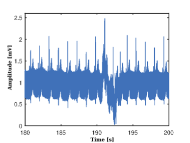
The result of the processing of the ECG signals extracted from the participants, the calculation of the RR series and their pre-processing can be analyzed from Figure 6, where Figure 6(a) shows the ECG signal, corresponding to one subject participating in the study, extracted from the Holter memory sampled at 225 Hz, visibly distorted by noise.
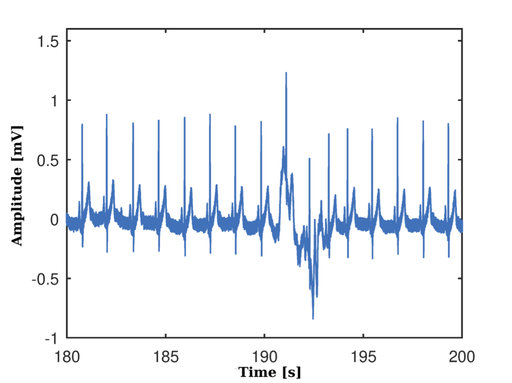
Subsequently, the signal processing is carried out in Figure 6(b), where the result of the application of the notch filter is observed, the elimination of the nonlinear trend in the signal and its subsequent oversampled at 1 KHz.
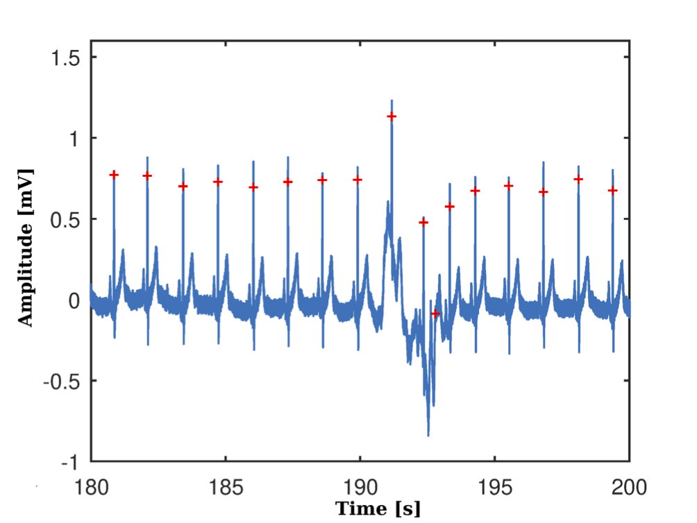
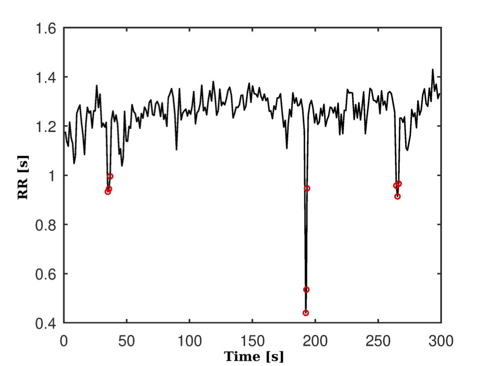
The results in the processing of the ECG signal to identify the peaks of the R waves and to this filtered signal are shown in Figure 7(a), while Figure 7(b) shows the RR series obtained, where some atypical beats are observed.
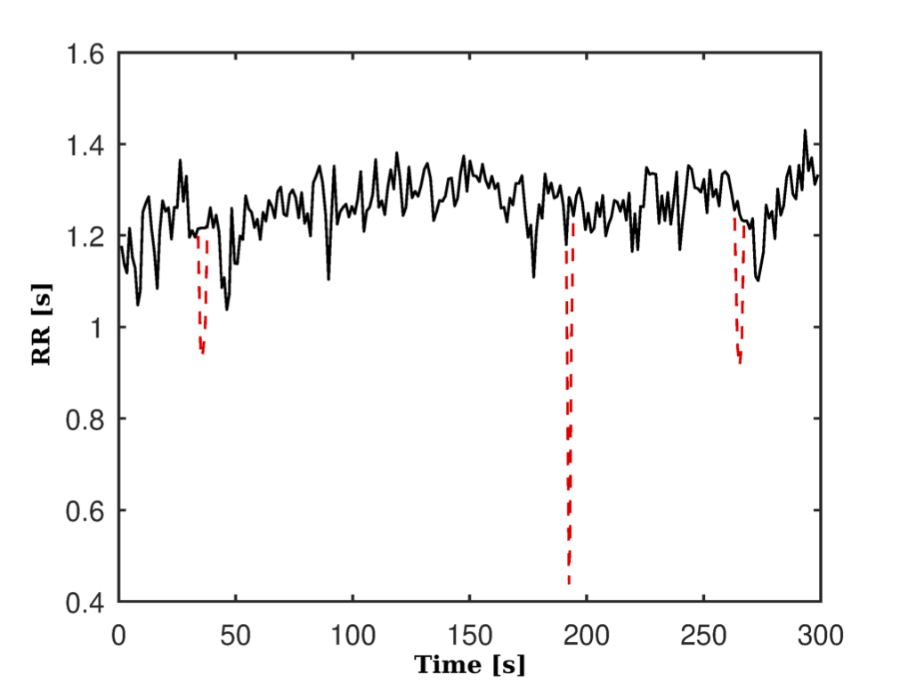
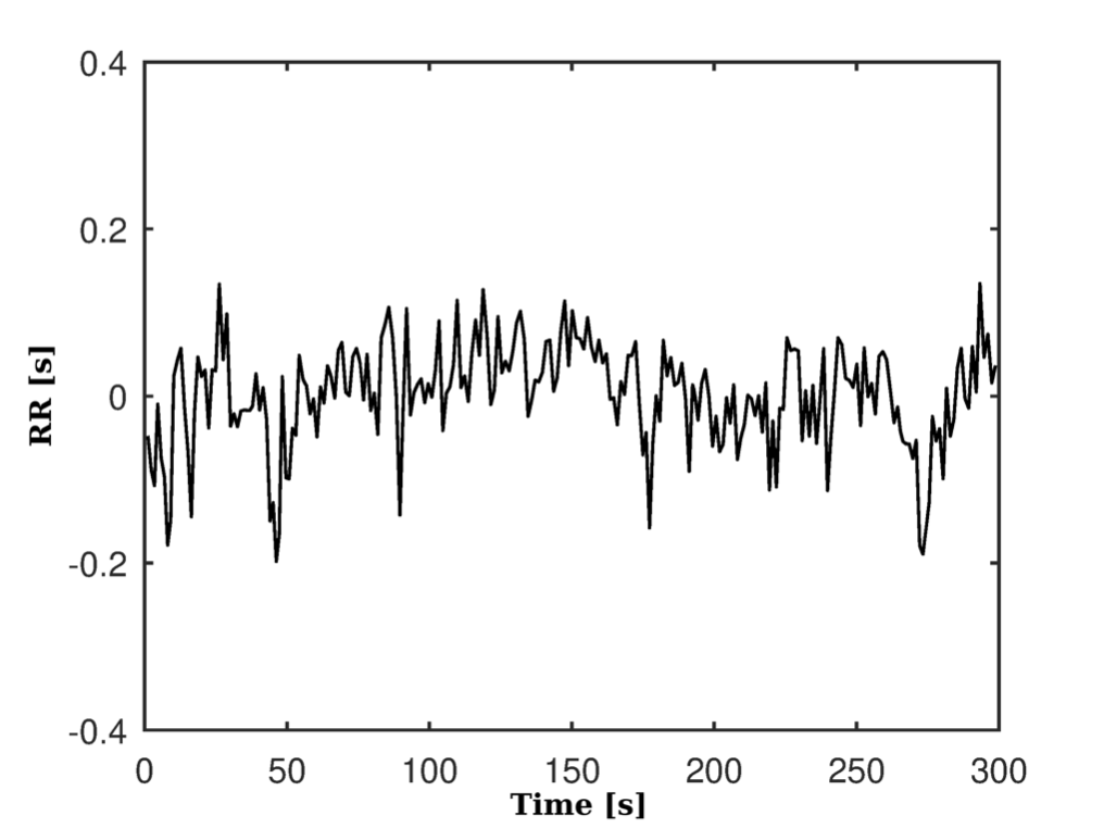
These artifacts were later corrected by interpolation. Figure 8(a) and Figure 8(b) respectively show the pre-processed series and without its linear trend and eliminating the continuous component.
| RR series | SS | SPS |
|---|---|---|
| 60 | 0.01 | 0.00 |
| 90 | 0.04 | 0.00 |
| 120 | 0.09 | 0.01 |
| 180 | 0.02 | 0.01 |
| 240 | 0.01 | 0.01 |
| 300 | 0.14 | 0.00 |
Table 1 shows the result of the Shapiro-Wilk normality test for each of the RR time series of the SS and SPS indicators. Table 2 presents the Spearman correlations of the GS series, on the one hand between the SS index and time (SDNN, RMSSD) and the frequency domain (LF, HF, LF/HF) and on the other the correlation between these indexes and the SPS index.
The observed correlation between LF/HF and SPS suggests a similar behavior for both indexes, as does the correlation between SD21 and SPS.
| Indexes | SS | SPS |
|---|---|---|
| RMSSD | -0.78** | -0.86** |
| SDNN | -0.77** | -0.77** |
| LF | -0.50* | -0.46* |
| HF | -0.72** | -0.78** |
| LF/HF | 0.39 | 0.60** |
| SD21 | 0.41 | 0.62** |
Table 3 shows the SS and SPS indicators of the RR series, whose values are given as medians and quartiles (1st; 3rd).
| RR series | SS | SPS |
|---|---|---|
| 60 | 13.61 (10.63 21.12) | 0.39 (0.21 1.26) |
| 90 | 14.10 (11.48 17.36) | 0.48 (0.23 1.07) |
| 120 | 13.48 (10.53 17.16) | 0.47 (0.24 1.05) |
| 180 | 13.18 (9.92 17.62) | 0.47 (0.23 1.09) |
| 240 | 13.47 (10.07 17.88) | 0.45 (0.24 1.01) |
| 300 | 12.87 (10.10 16.85) | 0.43 (0.25 0.96) |
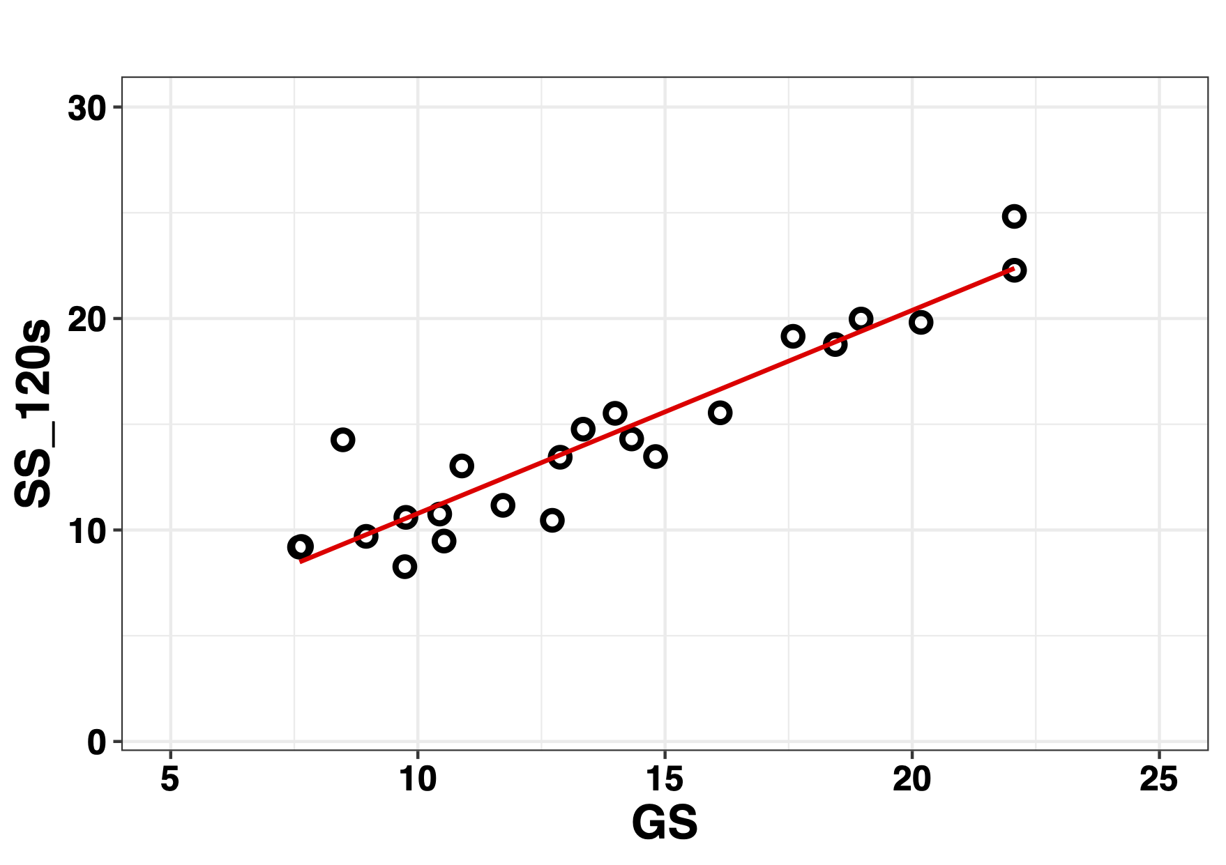
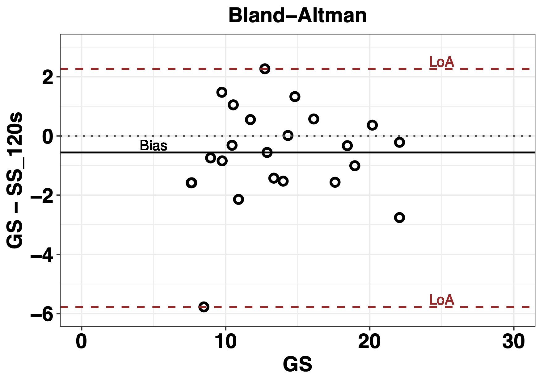
The correlation analysis of the series GS vs 120 s of the SS index is observed in the Figure 9. The analysis of the concordance between the series of 120 s and the GS by means of the Bland-Altman plot is shown in Figure 10, where the lines of bias are observed, the median of the difference between the series and the 2.5 and 97.5 percentiles of the LoA 95 %. GS is represented on the abscissa axis, not as traditionally, the average of the measurements [28].
| SS RR series (s) | Correlation (\(rho\)) (\(p\)) | Cliff (d) (c.i. 95%) | % error (\(e_{SS}\)) | Wilcoxon (\(p\)) | Bias (1st; 3rd) | LoA 95% |
|---|---|---|---|---|---|---|
| 300 vs 60 | 0.71 (1.98e-04) | 0.14 (-0.20 0.45) | 5.74 | 0.04 | -1.51 (-3.90 0.57) | -14.65 5.10 |
| 300 vs 90 | 0.84 (1.71e-06) | 0.16 (-0.18 0.48) | 9.48 | 0.02 | -1.04 (-2.56 0.35) | -6.67 1.89 |
| 300 vs 120 | 0.90 (3.28e-06) | 0.09 (-0.25 0.41) | 4.66 | 0.09 | -0.56 (-1.54 0.46) | -5.78 2.27 |
| 300 vs 180 | 0.96 (2.45e-06) | 0.06 (-0.28 0.38) | 2.37 | 0.03 | -0.58 (-1.36 0.35) | -3.90 1.61 |
| 300 vs 240 | 0.98 (1.99e-06) | 0.06 (-0.28 0.38) | 4.61 | 0.01 | -0.48 (-0.95 -0.07) | -3.23 1.40 |
The concordance analysis between GS and different time series of the SS index is presented in Table 4. Where an increase in the values of the Spearman correlation coefficients (rho) is observed with the temporal increase of the ultra-short series with value of \(0.90\) from the series of 120 s of SS index.
The resulting Cliff Delta (d) values are very small and considered insignificant for all series. Values of % error (\(e_ {SS}\)) that are not greater than 10 % are observed between the GS serie and each of the ultra-short series. An overestimation of GS is observed due to the negative result of the bias. And there is a decrease in the LoA 95% with the temporary increase of the ultra-short series.
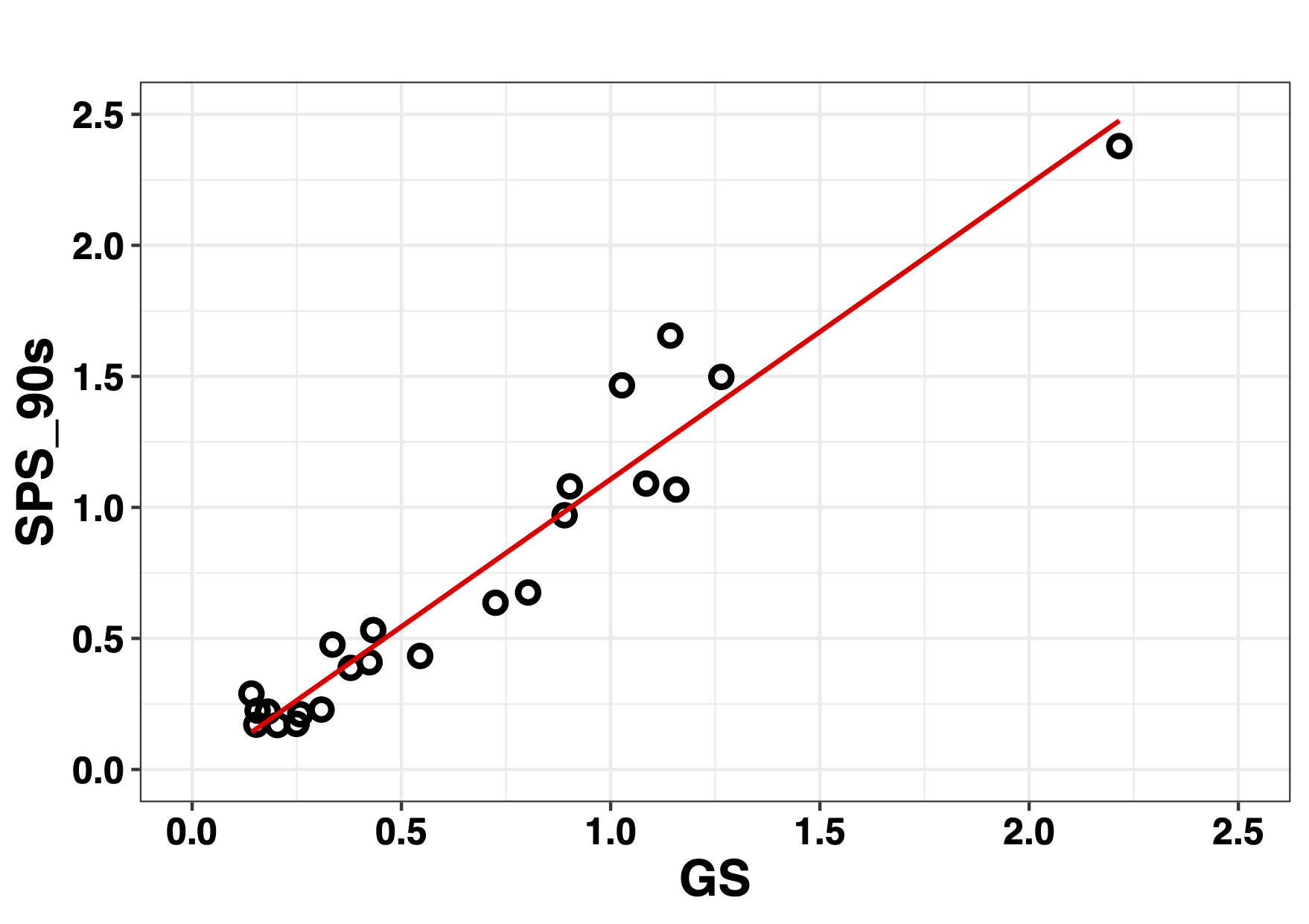
For the SPS index, Figure 11 shows the result of the correlation between the GS series and the ultra-short series of 90 s an accumulation of values below 0.5 of the GS series is observed in the graph.
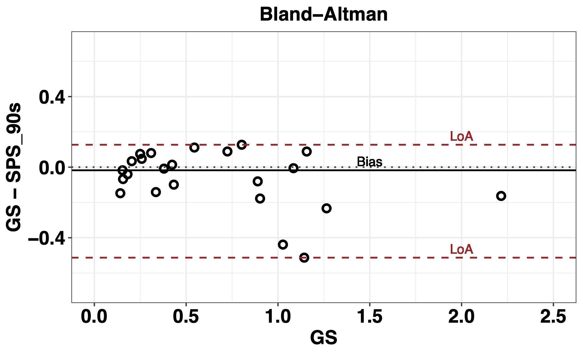
The analysis of the concordance of the GS and SPS of 90 s carried out using the Bland-Altman graph is shown in Figure 12 where it is possible to observe an overestimation of the GS due to the negative value resulting from the Bias in addition to an accumulation of negative values between 0 and 0.5 and a large asymmetry between the LoA.
| SPS RR series (s) | Correlation (\(rho\)) (\(p\)) | Cliff (d) (c.i. 95%) | % error (\(e_{SPS}\)) | Wilcoxon (\(p\)) | Bias (1st; 3rd) | LoA 95% |
|---|---|---|---|---|---|---|
| 300 vs 60 | 0.80 (7.02e-06) | 0.01 (-0.33 0.34) | 9.63 | 0.52 | -0.02 (-0.15 0.08) | -1.04 0.74 |
| 300 vs 90 | 0.93 (3.15e-06) | 0.05 (-0.28 0.38) | 10.15 | 0.15 | -0.02 (-0.14 0.06) | -0.51 0.13 |
| 300 vs 120 | 0.95 (2.79e-06) | 0.03 (-0.30 0.35) | 9.48 | 0.71 | 0.00 (-0.09 0.06) | -0.22 0.18 |
| 300 vs 180 | 0.98 (2.05e-06) | 0.05 (-0.29 0.372) | 8.85 | 0.29 | -0.02 (-0.08 0.03) | -0.32 0.22 |
| 300 vs 240 | 0.99 (1.71e-06) | 0.06 (-0.28 0.38) | 4.91 | 0.20 | -0.03 (-0.06 0.01) | -0.26 0.23 |
Table 5 shows the results of the methods used for the analysis of agreement between the GS and the ultra-short series corresponding to the SPS indicator. High Spearman values are observed mainly from the correlation between GS and the series of 90 s, \(rho=0.93\), \(p\) = 3.15e-06, reaching a value of \(rho=0.99\), \(p\) = 1.71e-06, for the correlation GS vs 240 s.
The Cliff Delta (d) shows negligible differences between the GS series, patron, and each of the ultra-short series of 60, 90, 120, 180 and 240 s. In the case of the % error (\(e_{SPS}\)), the is less than 10% in all cases. An overestimation of the GS series is observed, given by the negative value of the Bias, in addition the Wilcoxon test shows that the value of Bias could eventually be null. From the analysis of the Bland-Altman graph, it appears that the LoA 95% values decrease with the temporal increase of the ultra-short series, showing a greater degree of concordance between these series and the GS.
Discussion
The Poincaré graph is a simple method for evaluating HRV in the short term (5min) where, in addition, atypical RR intervals (premature beats, compensatory pauses or technical artifacts such as disconnection of electrodes, electromagnetic), influence the Poincaré trace with less force than in the analysis of the temporal and frequency domains [23], [29], [30].
The parameters extracted from the diagram SD1, SD2, separately, they are related to the linear domains of time and frequency [23], [31]. However, the relationship between the two, SD21, could be considered as an alternative measure to the autonomic balance indicator in the frequency domain LF/HF [4], [31], [32], and also presents a high correlation with non-linear HRV parameters, both in sick and healthy subjects [33]. Although it is not possible to establish a due metric mainly due to large inter-individual differences and statistical effects are shown on the group level [4], [29], [34].
The indicators SS and SPS, proposed by [16] provide reference values for the analysis of HRV in the short-term in elite soccer players and propose a interpretation to understand the physiological meaning of autonomic balance. Previous studies that have pointed out the importance of the reduction in measurement times to increase the use of HRV, especially in the daily clinic and analysis of sports performance in athletes. Using ultra-short HRV, records less than 5 min, [35] analyzed the SD21 indicator, establishing a minimum time required for its registration and [36] also using ultra-short HRV, they determined the minimum times for ultra-short registrations for SS and SPS.
The correlations found in this work, suggest on the one hand that SPS could be considered as an alternative for SD21 and also for LF/HF [37] and on the other that the behaviour of SS is similar to that found by [16].
For the analysis of the indicators, a method was used to reliably evaluate the equivalences between the series of the ultra-short HRV SS and SPS indicators and the short-term, 5 min. A value of \(rho = 0.90\) was adopted as the cutoff criterion, as a minimum, this threshold ensures that a measurement represents at least 81 % of the variability (\(rho ^ 2 = 0.81\)) an extremely low risk of committing a Type 1 error [10].
The results show a similarity in the values of the medians in the series of each index except for the series of 60 s, this is possibly due to the fact that this index requires a longer time window [29], in addition a positive increase in the values that reflect levels of agreement between the SS series and also in the series of the SPS indicator.
The threshold value proposed for the correlation in the SS index is observed from the 120 s series, negligible values are also observed for the Delta of Cliff and very low values of the error (\(e_{SS}\)). The ultra-short series of 180 and 240 s show a similar behaviour.
The analysis of the Bland-Altman graphs show high concordance from the GS series and the 120 s series, evidencing the similarity between the GS series and the ultra-short 180 s and 240 s, respectively. This allows to establish the equivalence of the series of 120 s with the GS for the index SS.
The analysis of the SPS indicator shows that from the 90 s series the criterion used is fulfilled, where \(rho = 0.93\), greater \(rho = 0.90\), here also the values of Cliff’s Delta are negligible, showing SPS equivalence with the GS from the ultra-short series of 90 s.
These findings can help us to understand, on the one hand, the usefulness of the Poincaré plot in the analysis of HRV, on the other hand, the decrease in recording time may allow an increase in the use of HRV for the analysis of the well-being of people.
These data should be interpreted with caution because the study had a small sample size. On the other hand, different stabilization times prior to the records were not analyzed. Furthermore, only the supine position was used for the ECG recordings and only the segment of the onset of the signal was analyzed. On the other hand, a single RR series pre-processing method was used.
It will be necessary to carry out more studies that take these variables into account.
Conclusions
In conclusion, the new SPS indicator proposed for the analysis of autonomic equilibrium could be considered as an alternative to the traditional LF / HF.
Furthermore, the ultra-short recordings of 120 s for SS, and 90 s for SPS, were equivalent to short-term HRV (5 min). The reduction in measurement times could possibly help increase the use of HRV to monitor the health and well-being and especially in the sports evaluation of large groups of athletes, by reducing the recording and processing times of the signals.
In future investigations, it might be possible to use these indicators in different populations and the use of different pre-processing methods.
Authors' Information
José Gallardo studied Electronics Engineering at the Universidad Tecnologica Nacional Facultad Buenos Aires, where he presented his Doctorate Thesis in Engineering. He also obtained a Master’s degree in Biomedical Engineering from the Universidad Nacional de Entre Rios. He is a Principal Professional at the Consejo Nacional de Investigaciones Cientificas y Tecnicas (CONICET) as well as professor and researcher at the Universidad de la Marina Mercante in Buenos Aires, Argentina.
Giannina Bellone has a degree in Psychology from the Universidad Catolica Argentina and a degree in Journalism. She is currently finishing her PhD in Science and Technology at the Universidad Nacional de Quilmes, Argentina. She is also a Specialist in Prevention of Occupational and Road Accidents and a researcher in the Chronophysiology Laboratory of BIOMED-UCA-CONICET. She is Professor of Labor Psychology in the Psychology career of the UCA.
Marcelo Risk is currently director of the Instituto de Medicina Traslacional e Ingenieria Biomedica associated with the Consejo Nacional de Investigaciones Cientificas y Tecnicas (CONICET), Istituto Universitario del Hospital Italiano de Buenos Aires and the Hospital Italiano de Buenos Aires, Argentina. He is also full-time professor at the Biomedical Engineering program at the Instituto Universitario Hospital Italiano de Buenos Aires. Mr. Marcelo Risk has a PhD from the Universidad de Buenos Aires, a ScD in Bioengineering from the Universidad Nacional de Córdoba, an MBA from the Universidad de Palermo, and a degree in Electronics Engineering from the Universidad Tecnologica Nacional, Argentina.
Authors' Contributions
José Gallardo participated in the research, methodology, software development as well as writing and reviewing the manuscript.
Giannina Bellone participated in the methodology, taking measurements, and reviewing the manuscript.
Marcelo Risk participated in the research, methodology, writing, and reviewing manuscript.
Competing Interests
The authors declare that they have no competing interests.
Funding
No funding was received for this project.