Introduction
Diffusion tensor imaging (DTI) in small animals is a framework that provides critical insights into brain anatomy in health and disease. The use of animal models allows monitoring of functional and fundamental cognitive aspects over time. Rats are among the most commonly used species for motor neurological modeling [1]–[3]. The rat’s motor circuits are homologous to many motor patterns in human primates, demonstrated by direct functional comparison [4], [5].
These facts open new possibilities to study the evolution of illnesses or degeneration processes associated with human motor-capabilities impairment and behavioral disorders, including, for example: Parkinson [6]–[8], Wallerian degeneration [9], [10], epilepsy [11], [12], schizophrenia [13]–[15] and multiple sclerosis [16], [17], among others. However, most DTI work in the field, including the references cited above, describes histological and biological studies with imaging support only in post-mortem stages.
Despite the apparent benefits of using animals in research, few references focus on in-vivo imaging analyses. Some of the main reasons for this apparent scarcity include setup difficulties such as:
Use of human scanning units or human fitted acquisition devices to scan small animals [18]
Differences in the positioning of the animals’ heads in volumetric coils [19]
Maintaining the animal’s head in a fixed position between acquisitions. Surface coils make the setup easier, but at the expense of an exponential degradation of image quality with increased distance from the coil [20].
The quality of the images is also affected by unavoidable vibrations produced in the acquisition system. Vibrations contribute with displacements of up to 1mm per axis every time a gradient is launched [21]. Recall that DTI uses diffusions gradients on top of positioning gradients,
Cardiac pulsations also contribute to image degradation [22]. Customized rat gating schemes lowering the dispersion in Fractional Anistropy (FA) and Mean Diffusivity (MD) readings by 24% and 12%, respectively, have been presented in [23]. According to [24], displacements on the order of 1mm per axis should be considered in non-gated acquisitions.
DTI reliability is highly dependent on the signal-to-noise ratio (SNR) [25], partial volume effects (PVE) [26], [27] and displacement artifacts [21], [23]. The influence of these image-quality deteriorating factors becomes critical when scanning small volumes due to the low spin recruitment rate, which is unavoidable when increasing spatial resolution. Moreover, as these deteriorating factors appear in the early stages of image creation, there are few possibilities to obtain a reliable diffusion estimation by software methods. Also, erroneous results are propagated all along the DTI pipeline.
Tractography, an representation of neuronal connectivity, second to diffusion estimation, is affected since algorithms that build the tracts from tensor models determine starting and stopping conditions from FA values [28].
Scientist in the animal neuro-modeling field has overlooked the inherent capabilities of the 2nd-rank diffusion model beyond geometric representation. They often work with low-quality images individually, although the nature of their research forces them to have multiple acquisitions of the same subjects in timely separated points. Here, we present abundant evidence showing that post-acquisition treatment can gradually improve image quality with each acquisition to a point where Tractography becomes reliable at very high resolution.
Materials and methods
Small animal data
DTI images on a single Wistar male rat were collected using a BioSpec 70/30 horizontal animal 7 Tesla scanner (Bruker BioSpin, Ettlingen, Germany) with a 12cm diameter inner cylinder. The MRI-receiver device is a phased array surface coil customized for rat skulls. The data consists of 18 experiments acquired with all combinations of the following acquisition parameters: b-values of 600, 1000, and 3000 s/mm\(^2\); one and three averages; voxel sizes of 0.2, 0.3, and 0.4mm\(^3\). This scheme leads to a total of 6 experiments per resolution. In all experiments, we estimate the diffusion using 30 gradient directions and 5 \(B_0\) images. TR/TE = 3150/31.6ms with a flip angle of 90° in a Spin Echo-DTI sequence. The images are all built with a FOV = 22.4 x 22.4 mm\(^2\) thus matrix dimensions are of 112 x 112, 72 x 72 and 56 x 56 for resolutions 0.2, 0.3 and 0.4 mm\(^3\) respectively.
All acquisitions are performed with the rodent’s head in a supine position and fixed with a tooth bar, ear bars, and adhesive tape. The operator supplies anesthetic gases (isoflurane in a mixture of 30% O\(_2\) and 70% N\(_2\)O) during the scans. In all acquisitions, the operator employed tripilot positioning readings to sharply locate the animal’s head in the magnet’s iso-center.
Acquisition times are different in each resolution and are presented in tables 1,2 and 3 in the results Section together with the SNR indexes of the raw data. Each used resolution defines the limits of a testing group. The methods explained here apply to each resolution separately. Animal work was conducted in compliance with the European Union directives on this topic.
Image preprocessing
The preprocessing comprehends two steps: skull-stripping and tensor estimation. For Skull stripping, we use an inverse-registration method, and the operator performed the following procedure at each resolution.
Select the subject with the best contrast-to-noise ratio (CNR) and label it as the model subject (MoD) for the resolution.
For each of the three MoD, a mask is manually drawn over a \(B_0\) image using ImageJ [29].
Perform linear registration using the \(B_0\) image from the MoD as moving data and the \(B_0\) image in each other subject as fixed data. The resulting transformation matrix (TM) is the operator that maps MoD acquisitions’ structures into the non-model ones.
Apply the TM to MoD mask to transport it to the space of the non-model acquisition. With this procedure, we reduce human interaction to drawing only one mask per resolution. After removing the non-brain tissues from the brain image, we generated tensors using MedINRIA [30].
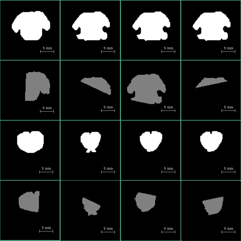
In some of the masks created during the skull stripping tasks, we found compelling evidence of rotations pivoting in the ears-fixing-bars and around the teeth bar (See Figure 1).
After carefully reviewing the setup and considering the multiple head fixing points in the current experiments, we concluded that the inter-acquisition rotations are due to unavoidable effects such as flexibility of the soft tissue in the mouth, ears, and the laxity of the jaw joint of the sedated animal. We fixed the linear displacements by software mechanisms, and we cite them in this manuscript as evidence of the difficulties in the setup. The reader is invited to keep in mind that the used resolution is in the order of some cents of a micrometer, which is far above the one used in humans; therefore, any minimal displacement in the setup crates significant misalignments in the images.
Core pipeline
Following suggestions in [26], [31], [32], multiple b-values are used: 600, 1000 and 3000 s/mm\(^2\). These values are the ones most often requested by researchers working with rat models in different pathology frameworks (see e.g. [33]–[35]). To correct the artifacts caused by head displacements, the transformation matrix (TM) resulting from an affine-linear registration in the FA-domain between the MoD and the other acquisitions is used to rotate the tensors coherently; therefore, aligning them to the underlying anatomy. With the structures aligned among acquisitions and willing to improve the CNR, we perform an averaging procedure in the tensor domain over all linearly registered experiments (see in Figure 2).
![Pipeline to improve image quality. First, we obtain the tensor information for each acquisition to generate the FA maps. Linear registration in the FA domain produces transformation matrices. The resulting transformation matrices are used to rotate the tensors and align them to the underlying anatomy [36]. Finally, we average all acquisitions to obtain images with enhanced quality. Note that all the images belong to the same subject; therefore, non-linear registration is not required.](assets/Figure1.png)
MedINRIA is used to execute the procedure in Figure 2 [37], which executes tensor estimation in the log-Euclidean space using a maximum likelihood criterion. The presented procedure has proven to be a successful strategy to avoid the tensor-size diminishing effect and non-positive tensors’ apparition. These effects usually appear when using direct algebraic methods in the presence of Rician noise [37].
Proof of concept
It is premised in this manuscript that a diffusion study is more cost and time effective if processing time is invested in the tensor-domain rather than in the DWI domain. We also stated that the use of the log-euclidean estimation strategy proposed in [37], is a good choice for the job since it avoids the creation of negative definite tensors. Finally, we claim that averaging tensors from multiple acquisitions enhance the quality of diffusion datasets. Fortunately, timely separated series of images is a standard scheme in animal frameworks. In this section, we settle all the theoretical basement to verify these postulates in a controlled environment. For this purpose, we create a synthetic diffusion structure from a diffusion-voxel-of-interest (DVOI) that is conveniently selected to demonstrate our postulates’ veracity. The DVOI contains one or several diffusion patterns, each one restricted to a cylinder of \(rho=5\) micrometers and length \(L=5\) millimeters, where the particles diffuse at \(1/1500 mm2/s\). We can voluntarily control the model’s diffusion pattern by rotating the vectorial components of the simulated signal. For convenience and without risk of losing generalization, the diffusion preference is modified only around the z-axis, and we force the reference diffusion to rest in the x-axis. To this end, the parameters \(\alpha\) in Equation [1] will be zero in the reference signal and might receive any value in the range [1,90] whenever willing to simulate non-perfectly overlapping diffusion signals among acquisitions.
\[fib_{i} = \left[cos(\alpha*\frac{pi}{180}), sin(\alpha*\frac{pi}{180}), 0 \right]; \label{}\]
For compatibility with the real data processing included in this manuscript, the simulated signals are studied with the same matrix of gradient directions mentioned in Section 2. Additionally, all the Diffusion Weighted Images (DWIs) in the DVOI are derived by extracting the log in both sides of the Sketjal-Tanner formulation as in Equation [2].
\[\log(\hat{S_{i}}) = \log(S_{o})-bg_{i}'Dg_{i} \label{eq:sketjal}\]
Where \(S_{o}\) is the non-sensitized signal, \(b\) the used b-value, \(g_{i}\) is the used gradient direction, \(D\) is the diffusion tensor and \(\hat{S_{i}}\) is the ith resulting DWI signal for each encoding \(g_{i}\) direction. The \(\hat{S_{i}}\) factor generalizes the cases where we work with ideal signals (\(N{1}\) and \(N_{2}\) in Equation [3] equal to zero) and also when modeling the signal affected by Rician noise (two independent Gaussians affecting \(S_{i}\)), in which case the value for \(\sigma\) will be explicitly given.
\[\hat{S_{i}} = \sqrt{[S_{i}+N_{1}(0,\sigma) + N_{2}(0,\sigma)} \label{eq:dwirician}\]
Then, we move the encoded D factors to the Log-euclidean (LE) domain where the tensor estimation is performed over \(\check{L}\) in Equation [4] using all existing DWI contributions.
\[D: L = \log(D) \rightarrow \check{L} \longleftrightarrow \check{D} = \exp(\check{L}) \label{eq:ledomain}\]
The LE domain operations provide positive definiteness and are computationally inexpensive. Finally, we move the tensor in the LE domain back to the euclidean domain as shown in Equation [4].
With this mathematical foundation, DWI signals are created and manipulated to reproduce rotational structural misalignments in ideal situations and the presence of Rician noise. Then, the pipeline depicted in Figure 2 is applied. A direct consequence of the simplified yet meaningful framework described in this section, is that rotations are forced to be in the x-y plane, therefore; rotational corrections are accomplished by \(T_{rot} = RTR'\) where \(R\) has the form defined in Equation [5].
\[R = \begin{bmatrix} \cos{\frac{\alpha*pi}{180}} & -\sin{\frac{\alpha*pi}{180}} & 0 \\ \sin{\frac{\alpha*pi}{180}} & \cos{\frac{\alpha*pi}{180}} & 0 \\ 0 & 0 & 1 \end{bmatrix} \label{eq:rotmat}\]
We use this exercise’s outcomes to generalize the method’s usefulness and clarify its effectiveness in real animal data. Figure 3 shows some of the synthetic material generated and used in the proof of concept.
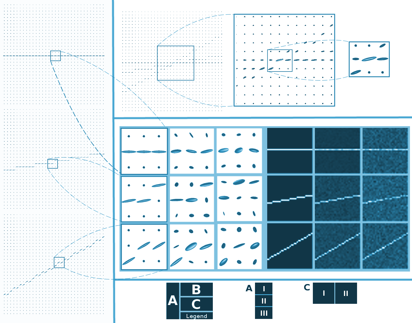
We use 32x32 pixels with a diffusion pattern crossing it as a reference in this proof of concept. From here, we extract a tensor, as shown in Panel AI. When required, different intentional rotations are induced in the tensor fields (see Panels A.II and A.III), and Rician noise with different levels is added (as evidenced in Panel CI). The created tensor fields can also create FA maps used for registration purposes as explained in Section 3.3. Thus, synthetic signals in DWI, fields in the tensor domain, and FA maps are available.
Application: corticospinal tract (CST) extraction in poor quality acquisitions
The CST is a bundle of axons that connects the spine to the cerebral cortex. Since humans and rats have similar anatomy of the central nervous system motor circuits, injuries in the CST in rats or humans lead to similar neurological symptoms: spasticity, increased deep tendon reflexes alongside decreased superficial reflexes, and loss of fine movements, among others. Longitudinal studies of the CST are of high pertinence since this tract is strongly affected after stroke in patients with motor sequelae [38]. Here, we use the CST structure to test whether it is possible to perform biologically meaningful Tractography in our improved images.
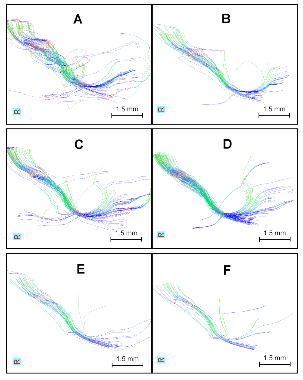
To extract the CST, we use the MoD acquisition to perform manual segmentation of the left primary motor cortex (Cx) and the left internal capsule (Ci). See Figure 4 for details. The resulting ROIs were propagated to other acquisitions using the registration process explained in Section 2.2. Then, the ROIs are used in MedINRIA as seeds to separate the tract of interest.
![Regions of interest for CNR measurements and tractography generation. Columns from left to right: Region of interest in the DWI, in the FA image and in a rat atlas. Upper row (A-C): the bundle of white matter pixels correspond to the internal capsule (CI). Bottom row (D-F): primary motor cortex (Cx). Atlas figures were adapted from [39].](assets/Figure2.png)
Data analysis and evaluation criteria in real animal data
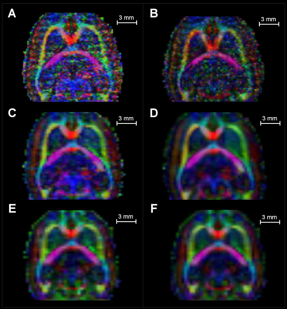
The qualitative improvement observed in FA color-coded maps (Figure 7) is quantitatively confirmed through a CNR metric in FA images (Figure 8). For the CNR computation, we use:
\[CNR = SNRWM_{} - SNR_{GM} = \frac{(S_{WM} - S_{GM})}{\delta}\]
SNRwm and SNRgm are the signal-to-noise ratios in the white and gray matter ROIs, respectively. \(S\) refers to signal while \(\delta\) stands for the standard deviation of the noise. We extracted these quantities by direct measurement in the background of the images that followed the same pipeline in Figure 2, but without applying the masking tasks.
We present the CNR metrics in a bar plot at each resolution (see Figure 8). Here, we analyze the whole data – time-domain averaged, and tensor-domain averaged – in the FA maps.
We performed Tractography using MedINRIA. For this purpose, the starting and the stopping conditions were defined using \(Start=min(FA_{WM})-\delta\) and \(Stop=min(FA_{GM})\), where FA stands for the fractional anisotropy index and subscripts WM and GM stands for white matter and gray matter respectively. We defined the starting and stopping conditions in the MoD and used them for fiber tracking in the MoD and the tensor-field-averaged image at each resolution, allowing for consistent comparison conditions.
Results
Pipeline in synthetic data
With the synthetic material produced as explained in Section 2.4, the proof of concept focused on the behavior of one centered pixel, where all the created signals converge -see Panel B in Figure 3 for referencing. The eigenvalues and eigenvectors that describe the diffusion geometry are dependent on how well overlapped are the concomitant diffusion patterns. Figures 5 and 6 register the results of these experiments.
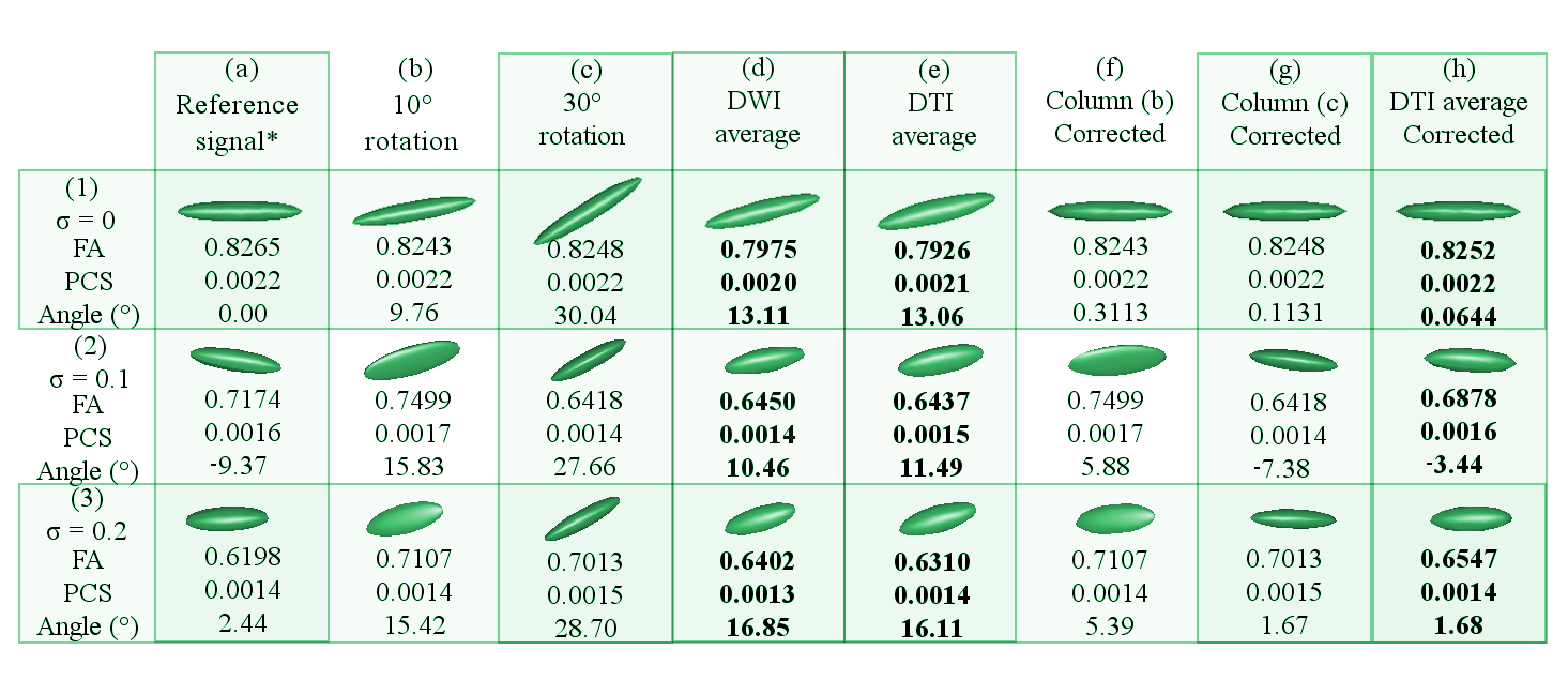
In Figure 5, Column (a) holds the tensor of the reference DWI signal. Columns (b) and (c) hold tensors of the DWI signals that have been 10and 30respectively, respect to the x-axis. Column (d) represents the tensor of the DWI signal that has been averaged within the DWI domain without any prior rotation correction. Column (e) shows the tensor averaged in the DTI domain with not rotational correction. Column (f) and (g) hold the corrected tensors of Columns (b) and (c), respectively. Column (h) displays the resulting tensor of averaging the tensors in Columns (a), (f) and (g). Row (1) shows the dataset with ideal conditions (no noise), row (2) dataset with 0.1 \(\sigma\), row (3) dataset with 0.2 \(\sigma\). The Angle() is the nearest angle (in degrees) of the principle eigenvector respect to the x-axis. Abbreviations: FA (fractional anisotropy); PCS (principal components); \(\sigma\) (variance of Rician noise). The symbol \(*\) is placed where the \(\sigma\) is 0.5 lower in the reference signals of the noisy datasets -rows 2 and 3-.
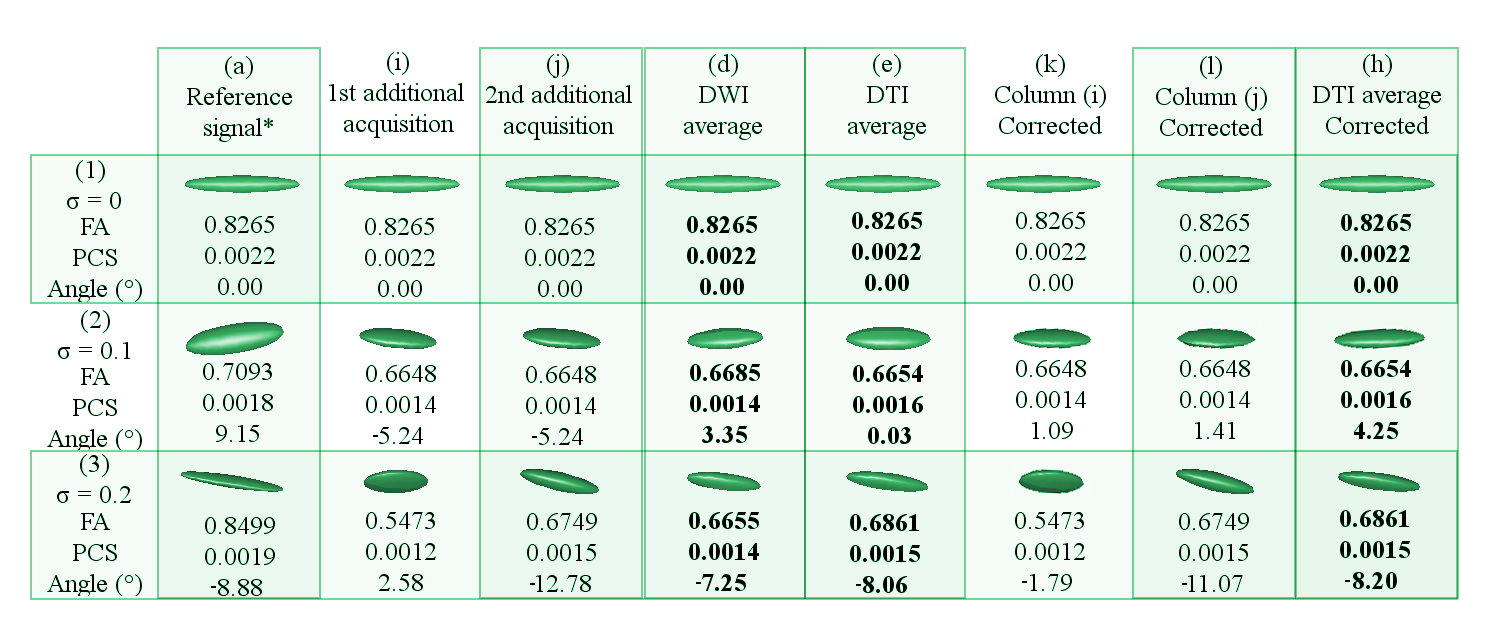
In Figure 6, Column (a) holds the tensor of the reference DWI signal. Column (i) and (j) contain tensors of the two additional DWI signals that have been randomly generated. Column (d) represents the tensor of the DWI signal that has been averaged within the DWI domain without any prior rotation correction. Column (e) shows the tensor in the DTI domain that has been derived from the DWI average in Column (d). Column (k) and (l) hold the corrected tensors of Columns (i) and (j), respectively. Column (h) displays the tensor that has been averaged from the tensors in Columns (f) and (g). Row (1) shows the dataset with ideal conditions (no noise), row (2) dataset with 0.1 \(\sigma\), row (3) dataset with 0.2 \(\sigma\). The Angle() is the nearest angle (in degrees) of the principle eigenvector respect to the x-axis. Abbreviations: FA (fractional anisotropy); PCS (principal components); \(\sigma\) (variance of Rician noise). The symbol \(*\) is placed where the \(\sigma\) is 0.5 lower in the reference signals of the noisy datasets -rows 2 and 3-.
Image quality in raw data and acquisition times
Before running the procedure described in methods, we run an SNR analysis in the raw data to determine if the data had the desired SNR level to execute a direct tractography.
| Parameters | SNR (\(B_0\)) | SNR(DWI) | Scan time |
|---|---|---|---|
| bv= 600 , avg = 1 | 2.32 ± 1.17 | 1.60 ± 0.73 | 00 : 40 : 50 |
| bv= 1000 , avg = 1 | 1.99 ± 1.34 | 1.01 ± 0.88 | 00 : 40 : 50 |
| bv= 3000 , avg = 1 | 2.23 ± 1.14 | 1.03 ± 0.39 | 00 : 40 : 50 |
| bv= 600 , avg = 3 | 3.08 ± 1.59 | 2.02 ± 0.98 | 02 : 02 : 30 |
| bv= 1000 , avg = 3 | 3.61 ± 1.91 | 1.92 ± 0.96 | 02 : 02 : 30 |
| bv= 3000 , avg = 3 | 3.03 ± 1.58 | 1.10 ± 0.42 | 02 : 02 : 30 |
| Parameters | SNR (\(B_0\)) | SNR(DWI) | Scan time |
|---|---|---|---|
| bv= 600,avg = 1 | 5.45 ± 2.97 | 3.48 ± 1.93 | 00 : 26 : 15 |
| bv= 1000,avg = 1 | 5.46 ± 2.93 | 2.73 ± 1.47 | 00 : 26 : 15 |
| bv= 3000,avg = 1 | 5.46 ± 2.93 | 1.42 ± 0.61 | 00 : 26 : 15 |
| bv= 600,avg = 3 | 9.09 ± 5.25 | 5.66 ± 3.44 | 01 : 18 : 45 |
| bv= 1000,avg = 3 | 9.48 ± 5.32 | 4.51 ± 2.71 | 01 : 18 : 45 |
| bv= 3000,avg = 3 | 9.23 ± 5.30 | 1.88 ± 0.96 | 01 : 18 : 45 |
| Parameters | SNR (\(B_0\)) | SNR(DWI) | Scan time |
|---|---|---|---|
| bv = 600, avg = 1 | 11.70 ± 6.91 | 6.83 ± 4.20 | 00 : 19 : 07 |
| bv = 1000, avg = 1 | 12.19 ± 7.12 | 5.48 ± 3.38 | 00 : 19 : 07 |
| bv = 3000, avg = 1 | 11.64 ± 6.07 | 2.24 ± 1.16 | 00 : 19 : 07 |
| bv = 600, avg = 3 | 20.18 ± 11.90 | 11.56 ± 7.20 | 00 : 57 : 21 |
| bv = 1000, avg = 3 | 20.62 ± 12.07 | 9.02 ± 5.75 | 00 : 57 : 21 |
| bv = 3000, avg = 3 | 19.99 ± 11.56 | 3.40 ± 1.96 | 00 : 57 : 21 |
In Tables 1, 2 and 3, SNR: signal to noise ratio in times, \(B_0\): group of images acquired with b-value=0, DWI: diffusion weighted images, bv: b-value in \(s/mm^2\), avg: scan averages.
The records in tables 1,2,3 show the SNR in raw data and scanning times for each acquisition. The values labeled \(B_0\) correspond to an average of the five non-sensitized volumes. Regarding the DWIs, we use the available 30 volumes in the averaging. Concerning SNR computation, we separate the needed signals with the skull stripping mask (see Section 2). As for the noise, we obtained it by inverting a dilated version of the skull-stripping mask; thus, the high-intensity pixels belonging to the skull are avoided. Most of the SNR mean values in Tables 1,2 and 3 are below 10, the level necessary for suitable DTI processing [39]. The only exception is the experiment acquired at a resolution of 0.4mm\(^3\) with three averages and a b-value of 600s/mm\(^2\). Hence, these typical MRI acquisitions for small animals render poor quality images.
Core pipeline for image improvement
The FA color-coded maps in Figure 7 show qualitatively how the images are improved for each resolution by following the procedure depicted in Figure 2. In all cases, the tensor-domain averaged image presented a better definition of structures and less noise than any individual MoD acquisitions on the left.
CNR measures in raw and processed data
Figure 8 shows the acquisition that differs only in the number of machine averages from the MoD with an arrow and labeled as homolog MoD (H.MoD). The difference between the H.MoD (One machine average) and the MoD (three machine averages) is the improvement obtained from the machine averaging procedure. The difference between the H.MoD and the results of processing all the data with one average at a given resolution (T-Avg_1) defines our method’s improvement ratio. This ratio also represents a fair comparison scheme with the machine averaging strategy since the three experiments used in T-Avg_1, consume the same acquisition time required for MoD generation at each resolution. The ratio of improvement in WM regions between MoD and the T-Avg_1 is 41% and 12.5% for resolutions \(0.3mm^3\) and \(0.4mm^3\), respectively.

The bars labeled as T-Avg_6 in Figure 8 show the incremental improvements achieved when using all the available data per resolution (6 scans). There is no average machine counterpart to compare these results to, given the excessively long acquisition time required for experiments using more than three machine averages (Ta>2h). This fact, perhaps superficial, highlights another contribution of our strategy by opening the possibility of using inter-acquisition information for image-enhancing purposes.
In Table 4, we show the SNR in the WM and GM obtained from FA maps at each resolution for images corresponding to H.MoD, MoD, and the tensor-domain processed image (T-Avg_1).
| Res (\(mm^3\)) | Zone | SNR readings | Improvement ratios | ||||
| H.MoD | MoD | T-Avg_1 | MoD/H.MoD | T-Avg_1/H.MoD | |||
| 0.2 | \(WM_{CI}\) | \(5.38\pm1.49\) | \(8.87\pm1.63\) | \(7.78\pm1.64\) | \(1.64\pm0.54\) | \(1.44\pm0.50\) | \(\downarrow\) |
| \(GM_{CX}\) | \(2.01\pm0.80\) | \(2.45\pm0.81\) | \(2.56\pm0.81\) | \(1.21\pm0.63\) | \(1.27\pm0.64\) | \(\uparrow\) | |
| 0.3 | \(WM_{CI}\) | \(8.84\pm2.17\) | \(11.97\pm3.14\) | \(17.07\pm2.88\) | \(1.35\pm0.48\) | \(1.93\pm0.57\) | \(\uparrow\) |
| \(GM_{CX}\) | \(3.98\pm1.10\) | \(4.64\pm1.20\) | \(6.23\pm2.16\) | \(1.19\pm0.45\) | \(1.60\pm0.71\) | \(\uparrow\) | |
| 0.4 | \(WM_{CI}\) | \(17.51\pm2.13\) | \(24.08\pm3.36\) | \(27.18\pm2.89\) | \(1.37\pm0.25\) | \(1.55\pm0.24\) | \(\uparrow\) |
| \(GM_{CX}\) | \(4.86\pm1.08\) | \(6.60\pm2.01\) | \(7.26\pm1.69\) | \(1.35\pm0.51\) | \(1.49\pm0.48\) | \(\uparrow\) | |
Application: Extraction of the CST tract
Finally, the CST is extracted using two ROIs, Ci and Cx. Figure 9 shows the extracted CST at each resolution. The best trade-off between voxel size and CNR is found when using voxels of 0.3mm\(^3\). Other voxel sizes present anatomically consistent results, but the number of fibers is reduced.
Discussion
The protocol presented in this manuscript generates reliable tractography in the low SNR regime common in small animal diffusion tensor images. We implemented an averaging strategy complemented with PVE and general misalignment’s offsetting procedures - as suggested in the literature [26],[27] [21],[23]- and improved the quality of small animal DTI images. Despite the low SNR in our native data (see tables 1,2,3), we were able to run Tractography on DTI acquired with voxels as small as \(0.2mm^3\) at 7T, and the procedure yielded anatomically consistent results.
The averaging process from the acquisition machine is a time-domain procedure applied in the DWI images. Our method applies the averaging in the tensor space where the geometry of the diffusion can be manipulated. We take advantage of this flexibility by rotating the tensors, therefore aligning them to the anatomy before performing the average.
We can not compare the two image-enhancing methods mentioned here, but they may be contrasted in terms of the results at the end or in a common stage of the pipeline. We decided to compare their performance in generating FA maps, which is of practical simplicity. We could have used the tensor fields for comparison purposes. However, their multivariate nature would lead to complex interpretations. In turn, the scalar nature of the FA maps allows direct reasoning. Moreover, since tractography defines its conditions in the FA maps, the improvement results are easily evidenced and correlated back and forward between the FA and the tractography domain.
We studied a set of different resolutions aiming to test the method’s response to different levels of noise. Our method outperformed the machine averaging in all cases except the 0.2mm\(^3\) resolution (see Figure 8), for which we found evidence suggesting that the lower performance is due to a lack of accuracy in the registration step and not to the level of noise. This spatial resolution dependency of the affine-registration-process accuracy has been reported in [40]. We plan to test different registration algorithms providing a quality assessment routine and add the possibility of choosing the desired registration algorithm to our codes.
Here, the improvements are limited by the inclusion of experiments done with b-values of 3000 s/mm\(^2\). While using high b-values highlight low-speed diffusion [41] and were included in our experiments to do a better diffusion estimation, the resulting images are highly noisy. The reader should expect even better improvement indexes when keeping the b-values lower than 2000 s/mm\(^2\).
Tensor estimation depends on the angular resolution used, and hence, one expects that the use of more gradient directions (GDs) would lead to better tensor estimations. Nevertheless, this dependency is not linear; thus, more GDs will not necessarily mean significantly better diffusion characterization [42], [43]. In our experience with small animals, using 6 GDs leads to over-estimation of the FA index in agreement with [44], but using more than 30 GDs (up to 126) does not create a remarkable difference in the FA readings. Since augmenting GDs increases the acquisition time, we decided to work with 30.
Data obtained at a resolution of 0.4mm\(^3\) is visually more robust during the whole process; however, the density of fibers at this resolution diminishes abruptly to the point of losing anatomical sense. This fiber density loss is due to the tensor model that allows for a single fiber per voxel (re-sampling techniques are not used); thus, images with bigger voxels will naturally display fewer fibers. Following this reasoning, the resolution of 0.2mm\(^3\) should have many more fibers than the other resolutions; besides, the low SNR in higher spatial resolution data generates overestimation of FA indices; thus, more pronounced preferences in diffusion directions. However, the Tensorlines algorithm in MedINRIA uses the angle of coincidence between adjacent voxels to connect lines [28]; therefore, the difficulty to integrate non-concomitant lines is a cause of tract scarcity in the 0.2mm\(^3\) resolution. The 0.3mm\(^3\) resolution gave the best improvements with our procedure, and displayed an excellent density of fibers in the image with improved SNR.
The acquisition protocol considered here uses only one subject that we scanned several times. Such a scheme avoids biological variability. In population studies, it is possible to extend the method to a multi-subject acquisition scheme. In that case, the procedure should include a non-linear registration step.
Conclusions
The most influential factor affecting image quality in small animals is the acquisition time. Increasing acquisition time touches practical aspects such as cost of service, availability of scanner and more importantly, ethics associated with the time that an alive subject might be inside the bore. The protocol presented in this manuscript facilitates the research groups’ work that requires small animal imaging services. Here we designed an image-enhancement alternative to the one built-in to scanners that improves image quality and allows for anatomically consistent Tractography.
We created this post-acquisition protocol knowing the crucial necessity of continued monitoring required in animal experimentation. In addition to improving the images with each time point –obtaining the entire profit of the scanning time and its associated costs– the protocol can be used to track changes. The mechanics of this change-tracking specification would be based in the same phenomena that cleans the images; if the data is not correlated between n time points, the averaging will lower the image’s intensity in the ROI (p.e. In neurodegenerative pathologies). Analogously, if a structure appears/grows in n time points, the averaging will increase the image’s intensity in the ROI (p.e. In brain plasticity events). Despite the idea introduced above is out of the scope of this manuscript, it has been recurrently proposed after witnessing our results and thus, will be part of a further extension of the methods explained here.
Authors’ Information
Juan Yepes Zuluaga obtained his B.Sc. in Computer Science from the University of Central Florida in 2020 and since then has been part of the development team that extends and supports Evalu@.
Fernando Yepes-Calderon obtained his B.Sc. in electronics in 2002 at Universidad del Valle, Colombia. Then, he worked in the telecommunications industry while pursuing a specialization in CISCO networking in 2003. He completed three masters: Biomedicine (Universidad de Los Andes, Colombia in 2007), Medical systems and computer science (INSA-Lyon, France in 2009), and Bioengineering (Universidad de Barcelona, Spain in 2011). In 2012 he registered for his Ph.D. at Universidad de Barcelona and moved to the United States to execute the research that ended in 2016 with several scientific publications and three patents. Doctor Yepes-Calderon has made contributions in Cancer, Alzheimer’s, Hydrocephalus, Sports in medicine, animal experimentation, and several industrial applications of artificial intelligence. Doctor Yepes-Calderon is the developer of Evalu@, the data centralizer for Artificial Intelligence applications.
Authors’ Contributions
Juan Yepes Zuluaga participated in the software validation, conceptualization, code testing, and writing, review, and editing the manuscript.
Fernando Yepes-Calderon participated in the research, conceptualization, code writing, methodology, project administration, writing the original draft, and writing, review, and editing the manuscript.
Competing Interests
The authors declare that they have no competing interests.
Funding
No funding was received for this project.
Availability of Data and Material
Post-processed images and derived data are available upon request. Please contact the corresponding author.
